LMM Tutorial

This tutorial walks through a complete LMM analysis. By the end, you will have:

Simulated longitudinal data with known parameters
Visualized individual trajectories
Fit and compared random intercept vs. random slope models
Interpreted fixed effects and variance components
Extracted and visualized individual trajectories (BLUPs)

Workflow Overview

┌─────────────────────────────────┐
│ 1. Setup                        │
│    Load packages, set seed      │
└────────────────┬────────────────┘
                 ▼
┌─────────────────────────────────┐
│ 2. Simulate/Load Data           │
│    Long format, check structure │
└────────────────┬────────────────┘
                 ▼
┌─────────────────────────────────┐
│ 3. Visualize                    │
│    Spaghetti plot, look first   │
└────────────────┬────────────────┘
                 ▼
┌─────────────────────────────────┐
│ 4. Fit Random Intercept Model   │
│    Baseline (parallel slopes)   │
└────────────────┬────────────────┘
                 ▼
┌─────────────────────────────────┐
│ 5. Fit Random Slope Model       │
│    Allow slopes to vary         │
└────────────────┬────────────────┘
                 ▼
┌─────────────────────────────────┐
│ 6. Compare Models               │
│    LRT, AIC/BIC                 │
└────────────────┬────────────────┘
                 ▼
┌─────────────────────────────────┐
│ 7. Check Diagnostics            │
│    Residuals, R², ICC           │
└────────────────┬────────────────┘
                 ▼
┌─────────────────────────────────┐
│ 8. Interpret Results            │
│    Fixed effects, variances     │
└────────────────┬────────────────┘
                 ▼
┌─────────────────────────────────┐
│ 9. Extract Random Effects       │
│    BLUPs, individual trajectories│
└─────────────────────────────────┘

Step 1: Setup

# Load packages
library(tidyverse)   # Data manipulation and plotting
library(lme4)        # Mixed models
library(lmerTest)    # p-values for lmer
library(performance) # R² and diagnostics
library(MASS)        # For mvrnorm (simulation)

# Set seed for reproducibility
set.seed(2024)

Step 2: Simulate Data

We'll create data with known population parameters so we can verify our model recovers them:

Parameter	True Value
Intercept mean (γ₀₀)	50
Slope mean (γ₁₀)	2
Intercept variance (τ₀₀)	100 (SD = 10)
Slope variance (τ₁₁)	1 (SD = 1)
I-S covariance (τ₀₁)	-2 (r ≈ -0.20)
Residual variance (σ²)	25 (SD = 5)

# Parameters
n_persons <- 200
time_points <- 0:4

# Fixed effects
gamma_00 <- 50  # Average intercept
gamma_10 <- 2   # Average slope

# Random effects covariance matrix
tau <- matrix(c(100, -2,
                -2,   1), nrow = 2)

# Residual SD
sigma <- 5

# Generate random effects for each person
random_effects <- mvrnorm(n = n_persons, mu = c(0, 0), Sigma = tau)
u0 <- random_effects[, 1]  # Random intercepts
u1 <- random_effects[, 2]  # Random slopes

# Generate data in LONG format (one row per observation)
data_long <- expand_grid(
  id = 1:n_persons,
  time = time_points
) %>%
  mutate(
    u0_i = u0[id],
    u1_i = u1[id],
    y = gamma_00 + u0_i + (gamma_10 + u1_i) * time + rnorm(n(), 0, sigma)
  ) %>%
  select(id, time, y)

# Check structure
head(data_long, 10)

✅ Checkpoint: You should see a tibble with columns id, time, and y. Each person has 5 rows (one per time point). Values will differ due to random generation, but y should be roughly in the 30–70 range.

# A tibble: 10 × 3
      id  time     y
   <int> <int> <dbl>
 1     1     0  61.2
 2     1     1  62.8
 3     1     2  65.1
 4     1     3  66.4
 5     1     4  69.2
 6     2     0  44.3
 7     2     1  47.8
 8     2     2  50.1
 ...

Step 3: Visualize

Always plot before modeling.

# Spaghetti plot: all individual trajectories
ggplot(data_long, aes(x = time, y = y, group = id)) +
  geom_line(alpha = 0.2, color = "gray40") +
  scale_x_continuous(breaks = 0:4, labels = paste("Time", 0:4)) +
  labs(x = "Time", y = "Score",
       title = "Individual Growth Trajectories",
       subtitle = paste("N =", n_persons, "participants")) +
  theme_minimal()

What to look for:

General trend (up, down, flat?)
Spread at baseline (intercept variance)
Fan pattern (slope variance)—do lines diverge or stay parallel?
Nonlinearity (curves vs. straight lines)
Outliers

# Add mean trajectory
mean_trajectory <- data_long %>%
  group_by(time) %>%
  summarise(mean_y = mean(y), .groups = "drop")

ggplot(data_long, aes(x = time, y = y)) +
  geom_line(aes(group = id), alpha = 0.15, color = "gray40") +
  geom_line(data = mean_trajectory, aes(y = mean_y),
            color = "steelblue", linewidth = 1.5) +
            # Note: ggplot2 < 3.4 used 'size' instead of 'linewidth'
  geom_point(data = mean_trajectory, aes(y = mean_y),
             color = "steelblue", size = 3) +
  scale_x_continuous(breaks = 0:4) +
  labs(x = "Time", y = "Score",
       title = "Individual Trajectories with Mean Overlay") +
  theme_minimal()

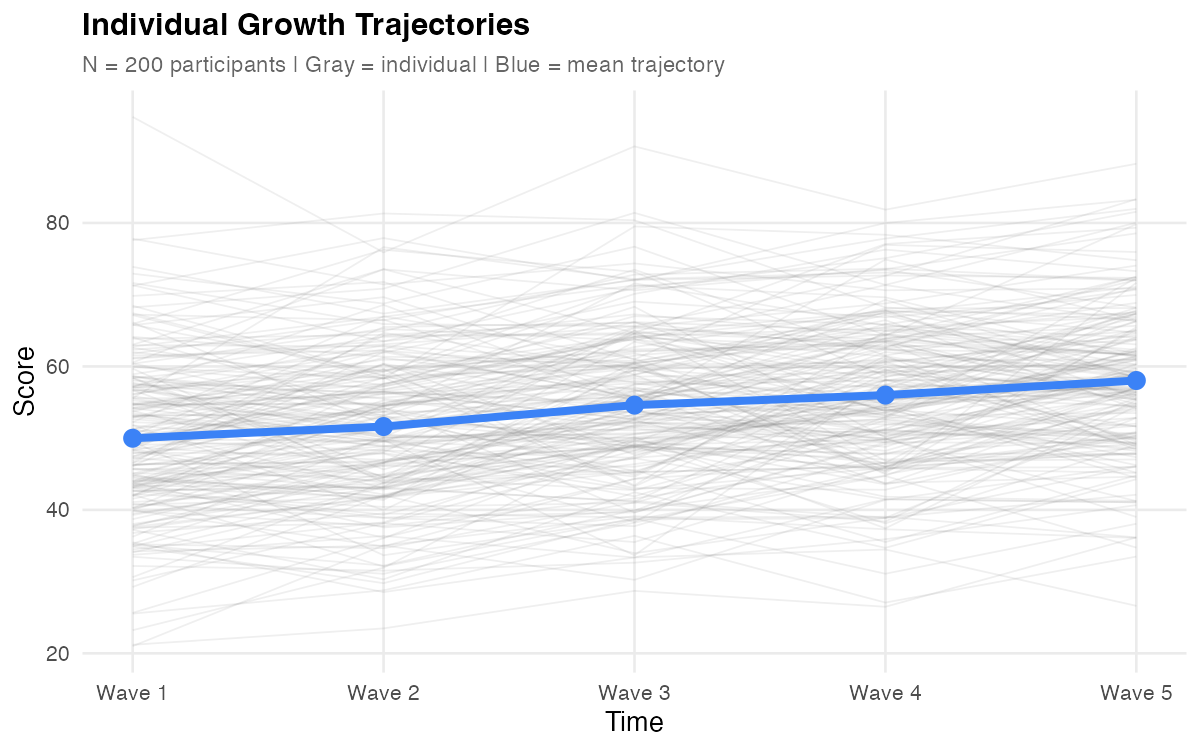
Figure: Individual trajectories (gray) with mean trajectory overlay (blue). The upward trend shows positive average growth; the spread shows individual differences.

✅ Checkpoint: Your plot should show upward-trending lines with visible spread at baseline and a slight "fan" pattern over time (lines diverging, indicating slope variance).

Step 4: Fit Random Intercept Model

Start with a baseline model: random intercepts only (slopes fixed across people).

mod_ri <- lmer(y ~ time + (1 | id), data = data_long)

summary(mod_ri)

Expected output (key sections):

Random effects:
 Groups   Name        Variance Std.Dev.
 id       (Intercept) 85.2     9.23
 Residual             45.3     6.73
Number of obs: 1000, groups:  id, 200

Fixed effects:
            Estimate Std. Error      df t value Pr(>|t|)
(Intercept)  49.856      0.712  198.00   70.02   <2e-16 ***
time          2.014      0.067  799.00   30.06   <2e-16 ***

Note: Your exact values will differ slightly due to random sampling, but the patterns should match.

What this model assumes:

People differ in their starting level (random intercepts)
Everyone changes at the same rate (fixed slope)
Lines are parallel

Note: This model forces everyone to have the same slope. The "missing" slope variance gets absorbed into the residual—notice the residual variance (45.3) is larger than the true value (25).

Step 5: Fit Random Slope Model

Now allow slopes to vary across individuals.

mod_rs <- lmer(y ~ time + (1 + time | id), data = data_long)

summary(mod_rs)

Expected output (key sections):

Random effects:
 Groups   Name        Variance Std.Dev. Corr
 id       (Intercept) 98.54    9.93
          time         0.89    0.94     -0.18
 Residual             24.89    4.99
Number of obs: 1000, groups:  id, 200

Fixed effects:
            Estimate Std. Error       df t value Pr(>|t|)
(Intercept)  49.923      0.732  199.000   68.21   <2e-16 ***
time          2.021      0.085  199.000   23.78   <2e-16 ***

What this model adds:

Each person has their own intercept AND slope
Lines can have different starting points and different angles (non-parallel)
The intercept-slope correlation (-0.18) indicates higher starters tend to have slightly flatter slopes

Compare Estimates to True Values

Parameter	True Value	Estimate
Intercept mean	50	49.92
Slope mean	2	2.02
Intercept variance	100	98.54
Slope variance	1	0.89
I-S correlation	-0.20	-0.18
Residual variance	25	24.89

Numbers shown are illustrative from one simulated run; your results will differ with seed, RNG, and package versions.

✅ Checkpoint: Estimates closely recover the true population parameters. This confirms the model is working correctly.

Step 6: Compare Models

Is the random slope model significantly better than random intercept only?

# Use ML for model comparison (not REML)
mod_ri_ml <- lmer(y ~ time + (1 | id), data = data_long, REML = FALSE)
mod_rs_ml <- lmer(y ~ time + (1 + time | id), data = data_long, REML = FALSE)

anova(mod_ri_ml, mod_rs_ml)

Expected output:

Data: data_long
Models:
mod_ri_ml: y ~ time + (1 | id)
mod_rs_ml: y ~ time + (1 + time | id)
          npar    AIC    BIC  logLik deviance  Chisq Df Pr(>Chisq)
mod_ri_ml    4 6234.5 6254.1 -3113.2   6226.5
mod_rs_ml    6 6142.8 6172.2 -3065.4   6130.8 95.68  2  < 2.2e-16 ***

The random slope model fits significantly better (p < .001).

Use ML (REML = FALSE) for model comparisons (AIC/BIC, LRT); use REML for final parameter estimation.

Information Criteria

data.frame(
  Model = c("Random Intercept", "Random Slope"),
  AIC = c(AIC(mod_ri_ml), AIC(mod_rs_ml)),
  BIC = c(BIC(mod_ri_ml), BIC(mod_rs_ml))
) %>%
  mutate(across(where(is.numeric), \(x) round(x, 1)))
  # Note: R < 4.1 use function(x) instead of \(x)

✅ Checkpoint: Both AIC and BIC should favor the random slope model (lower values = better fit).

Step 7: Check Diagnostics

Before interpreting results, verify model assumptions.

Residual Plots

# Residuals vs. fitted
plot(mod_rs)

# Q-Q plot for residuals
qqnorm(resid(mod_rs))
qqline(resid(mod_rs))

# Q-Q plot for random intercepts
qqnorm(ranef(mod_rs)$id[,1])
qqline(ranef(mod_rs)$id[,1])

What to look for:

Diagnostic	Good	Problematic
Residuals vs. fitted	Random scatter around 0	Funnel shape, curves
Q-Q plot (residuals)	Points on line	Heavy tails, skewness
Q-Q plot (random effects)	Points on line	Heavy tails (less critical)

Examine Residuals vs Fitted (random scatter) and Normal Q-Q (approximate line). Heavier tails in random-effects Q-Q are common and typically less critical.

Check for Singular Fit

isSingular(mod_rs)  # Should be FALSE

A singular fit warning means a variance component is estimated at zero—often indicating an over-specified model.

If singular: try removing the random slope, rescaling or centering time, or collecting more waves; for Bayesian fits, consider informative priors.

Variance Explained (R²)

r2(mod_rs)

Interpretation:

Marginal R²: Variance explained by fixed effects (time) alone
Conditional R²: Variance explained by fixed + random effects

Typical values: Marginal R² might be 0.10–0.30 (time explains some variance); Conditional R² is usually much higher (0.70–0.90) because individual differences explain most variation.

Intraclass Correlation (ICC)

From the random intercept model:

icc(mod_ri)

ICC ≈ 0.65 means 65% of total variance is between persons (stable individual differences), and 35% is within persons (change over time + noise). This justifies using mixed models—there's meaningful clustering to account for.

With random slopes, ICC varies with time; the one-number ICC reported here comes from the random-intercept model and serves as a baseline clustering index.

✅ Checkpoint: Residual plots should show no obvious patterns. R² conditional should be high. ICC should justify the random intercept.

Step 8: Interpret Results

Fixed Effects

# Fixed effects with confidence intervals
fixef(mod_rs)
confint(mod_rs, parm = "beta_", method = "Wald")

We use Wald CIs for speed; profile CIs can be more accurate but are slower.

Parameter	Estimate	95% CI	Interpretation
Intercept	49.92	[48.49, 51.36]	Average score at Time 0
Slope	2.02	[1.85, 2.19]	Average change per time unit

"On average, participants started at 49.92 and increased by 2.02 units per time point."

Variance Components

VarCorr(mod_rs)

Component	Variance	SD	Interpretation
Intercept	98.54	9.93	People differ in starting level (SD ≈ 10)
Slope	0.89	0.94	People differ in rate of change (SD ≈ 1)
Correlation	-0.18	—	Higher starters grow slightly slower
Residual	24.89	4.99	Occasion-specific noise (SD ≈ 5)

Intercept-Slope Correlation

The correlation of -0.18 is small—higher starters grew slower, but most still improved. This is a common pattern: those who start high have less room to grow (or regress toward the mean).

Proportion with Positive Slopes

A positive slope mean doesn't mean everyone improved. Check:

slope_mean <- fixef(mod_rs)["time"]
slope_sd <- sqrt(VarCorr(mod_rs)$id["time", "time"])

# P(slope > 0) — theoretical
pnorm(0, mean = slope_mean, sd = slope_sd, lower.tail = FALSE)
# ≈ 0.98

# Empirical share with positive slopes using BLUPs
re <- ranef(mod_rs)$id
mean(fixef(mod_rs)["time"] + re$time > 0)
# Should be close to the theoretical value

✅ Checkpoint: ~98% of participants had positive slopes. With slope mean ≈ 2 and SD ≈ 1, almost everyone improved. The BLUP-based share should be close to the theoretical pnorm() result.

Step 9: Extract Random Effects

Best Linear Unbiased Predictors (BLUPs)

The random effects for each person:

# Extract random effects
re <- ranef(mod_rs)$id
head(re)

   (Intercept)        time
1    11.234      0.512
2    -5.891     -0.234
3     2.156      0.089
...

These are BLUPs (conditional modes): person-specific deviations that are partially pooled toward the group mean.

Individual Trajectories

# Person-specific intercepts and slopes
person_effects <- data.frame(
  id = 1:n_persons,
  intercept = fixef(mod_rs)["(Intercept)"] + re$`(Intercept)`,
  slope = fixef(mod_rs)["time"] + re$time
)

head(person_effects)

Plotting Individual Predictions

# Get fitted values
data_long$fitted <- fitted(mod_rs)

# Plot a subset of individuals
sample_ids <- sample(unique(data_long$id), 30)

data_long %>%
  filter(id %in% sample_ids) %>%
  ggplot(aes(x = time, y = fitted, group = id)) +
  geom_line(alpha = 0.6, color = "steelblue") +
  geom_point(aes(y = y), alpha = 0.4, size = 1) +
  labs(x = "Time", y = "Score",
       title = "Model-Implied Trajectories for 30 Participants",
       subtitle = "Lines = fitted trajectories; Points = observed data") +
  theme_minimal()

Shrinkage Visualization

A key advantage of mixed models is shrinkage—extreme individual estimates are pulled toward the group mean. Compare BLUPs to OLS estimates:

# OLS estimates for each person (no pooling)
ols_estimates <- data_long %>%
  group_by(id) %>%
  summarise(
    ols_intercept = coef(lm(y ~ time, data = pick(everything())))[1],
    ols_slope     = coef(lm(y ~ time, data = pick(everything())))[2],
    .groups = "drop"
  )

# Combine with BLUPs
comparison <- person_effects %>%
  left_join(ols_estimates, by = "id")

# Plot shrinkage for intercepts
ggplot(comparison, aes(x = ols_intercept, y = intercept)) +
  geom_point(alpha = 0.5) +
  geom_abline(slope = 1, intercept = 0, linetype = "dashed", color = "red") +
  geom_vline(xintercept = fixef(mod_rs)["(Intercept)"],
             linetype = "dotted", color = "gray50") +
  geom_hline(yintercept = fixef(mod_rs)["(Intercept)"],
             linetype = "dotted", color = "gray50") +
  labs(x = "OLS Estimate (No Pooling)",
       y = "BLUP Estimate (Partial Pooling)",
       title = "Shrinkage of Individual Intercepts",
       subtitle = "Points below diagonal = shrinkage toward mean") +
  theme_minimal()

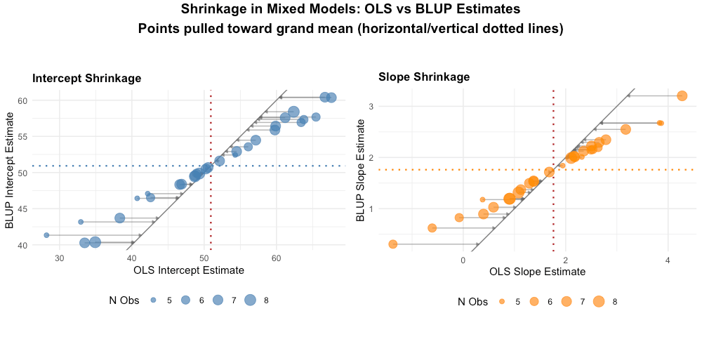
Figure: Shrinkage demonstration. Points near the dashed red line (y = x) show little shrinkage. Points pulled toward the grand mean (dotted lines) show substantial shrinkage—these are typically individuals with extreme OLS estimates.

Key observations:

Extreme OLS estimates are pulled toward the grand mean
The degree of shrinkage depends on how extreme the estimate is and data reliability
This "borrowing of strength" across individuals is a core advantage of mixed models

Written Summary

We estimated a linear mixed model for 200 participants across 5 time points. Adding random slopes significantly improved fit over a random-intercept-only model (χ²(2) = 95.68, p < .001; ΔAIC = 91.7).

On average, participants started at 49.92 (SE = 0.73, 95% CI [48.49, 51.36]) and increased by 2.02 units per time point (SE = 0.09, 95% CI [1.85, 2.19]), both p < .001. Significant individual differences emerged in starting levels (SD = 9.93) and growth rates (SD = 0.94). The negative intercept-slope correlation (r = -0.18) indicates that participants who started higher grew slightly slower.

The model explained substantial variance (conditional R² ≈ 0.80), with most variance attributable to stable individual differences (ICC ≈ 0.65).

Complete Script

# ============================================
# LMM Complete Worked Example
# ============================================

# Setup
library(tidyverse)
library(lme4)
library(lmerTest)
library(performance)
library(MASS)
set.seed(2024)

# Simulate data
n_persons <- 200
gamma_00 <- 50; gamma_10 <- 2
tau <- matrix(c(100, -2, -2, 1), nrow = 2)
sigma <- 5

random_effects <- mvrnorm(n_persons, c(0, 0), tau)
u0 <- random_effects[, 1]; u1 <- random_effects[, 2]

data_long <- expand_grid(id = 1:n_persons, time = 0:4) %>%
  mutate(
    y = gamma_00 + u0[id] + (gamma_10 + u1[id]) * time + rnorm(n(), 0, sigma)
  )

# Visualize
ggplot(data_long, aes(x = time, y = y, group = id)) +
  geom_line(alpha = 0.2) +
  theme_minimal() +
  labs(title = "Individual Trajectories")

# Fit models
mod_ri <- lmer(y ~ time + (1 | id), data = data_long)
mod_rs <- lmer(y ~ time + (1 + time | id), data = data_long)

# Compare models (use ML)
mod_ri_ml <- lmer(y ~ time + (1 | id), data = data_long, REML = FALSE)
mod_rs_ml <- lmer(y ~ time + (1 + time | id), data = data_long, REML = FALSE)
anova(mod_ri_ml, mod_rs_ml)

# Diagnostics
plot(mod_rs)
isSingular(mod_rs)
r2(mod_rs)
icc(mod_ri)

# Final results
summary(mod_rs)
fixef(mod_rs)
VarCorr(mod_rs)
confint(mod_rs, parm = "beta_", method = "Wald")

# Extract random effects (BLUPs)
re <- ranef(mod_rs)$id
head(re)

Adapt to Your Data

To use this workflow with your own dataset:

1. Read and Prepare Data

LMM requires long format: one row per observation.

library(readr)
library(tidyr)

# If your data is in WIDE format (one row per person):
data_wide <- read_csv("my_data.csv")  # columns: id, y_t1, y_t2, y_t3, y_t4, y_t5

# Convert to long format
data_long <- data_wide %>%
  pivot_longer(
    cols = starts_with("y_t"),
    names_to = "wave",
    names_prefix = "y_t",
    values_to = "y"
  ) %>%
  mutate(time = as.numeric(wave) - 1)  # Code time as 0, 1, 2, 3, 4

2. Check Time Variable

Time must be numeric for growth models:

class(data_long$time)  # Should be "numeric" or "integer"

# If it's a factor with numeric labels (e.g., "0","1","2"):
data_long$time <- readr::parse_number(as.character(data_long$time))

3. Update Model Formula

Replace variable names as needed:

mod <- lmer(outcome ~ time + (1 + time | participant_id), data = data_long)
summary(mod)

✅ Checkpoint: Once your basic model runs, layer on diagnostics, model comparisons, and random effects extraction exactly as shown above. See the Reference for time coding options if your waves are unequally spaced.

Next Steps

Need syntax or thresholds? → Reference
Hit an error? → Reference: Troubleshooting
Back to overview → LMM Guide