Why Mixed Models?
When you measure the same people repeatedly, your observations aren't independent. A person who scores high at Time 1 is more likely to score high at Time 2. Standard regression ignores this, leading to:
- Inflated confidence in your estimates
- Misleading p-values
- No way to model individual differences in change
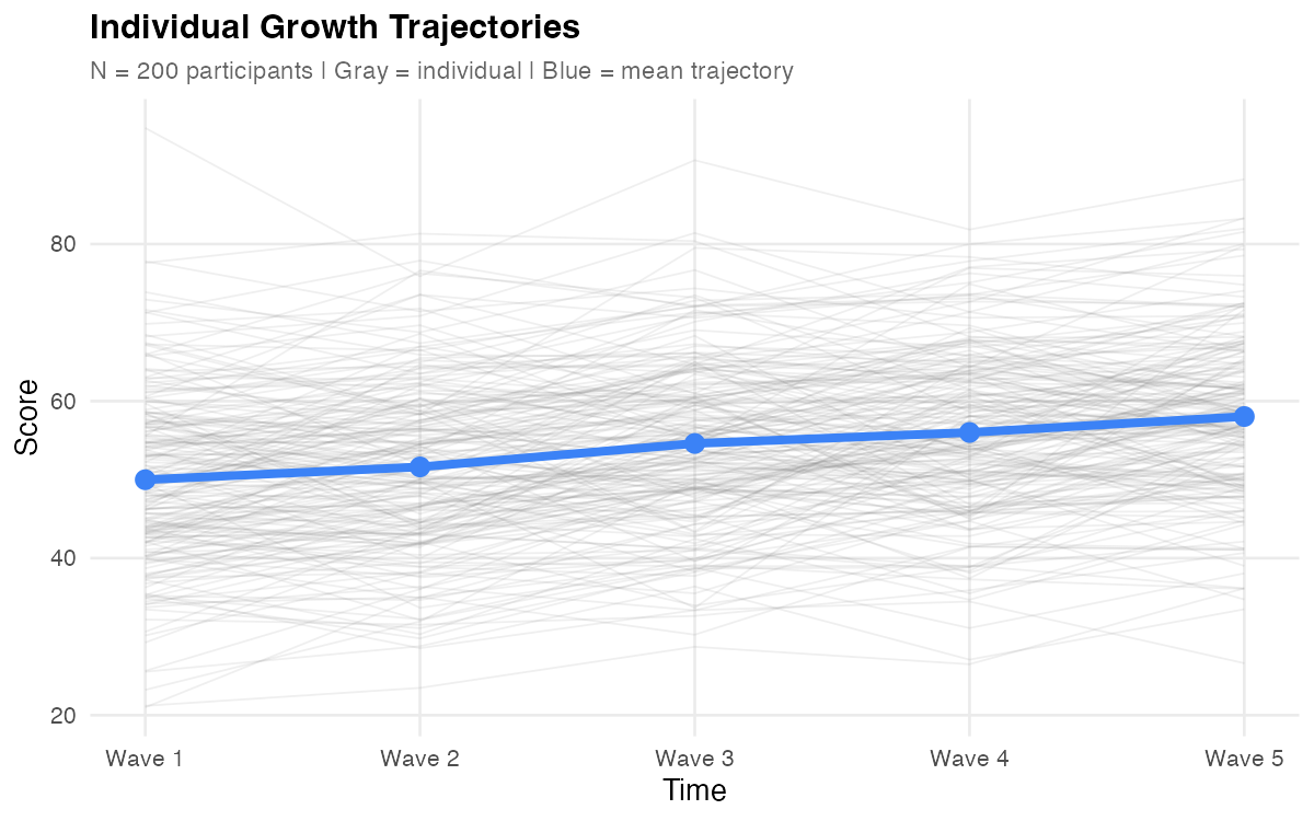
Consider 200 participants measured at 5 time points each. You have 1,000 observations, but they're not 1,000 independent pieces of information—the 5 observations from Person 1 are more similar to each other than to observations from Person 47.
The mean tells you "the group improved"—but the real questions are about the spread: How much do starting points vary? Do people change at different rates? Standard approaches handle these poorly:
| Approach | What It Does | Problem |
|---|---|---|
| Ignore nesting | Treat all 1,000 observations as independent | SEs too small, p-values too optimistic |
| Aggregate | Compute person-means, analyze 200 means | Loses within-person information about change |
| Repeated measures ANOVA | Model time as fixed factor | Assumes sphericity (often violated); historically easier with balanced data |
| Mixed models | Model between- and within-person variation | Appropriate standard errors; individual trajectories |
Linear Mixed Models (LMM) solve this by explicitly modeling the dependency structure. The "mixed" refers to a mixture of:
- Fixed effects: Parameters that apply to everyone (average intercept, average slope)
- Random effects: Parameters that vary across individuals (person-specific deviations)
Quick mental model: Think of LMM as "fit one regression line per person, then summarize those lines." Each individual gets their own intercept and slope, but these estimates are informed by the whole sample—extreme values get pulled toward the group average, and people with sparse data borrow strength from others.
Look at the spaghetti plot above. Before reading further, consider:
- Intercept spread: How much do starting points vary at Wave 1?
- Slope divergence: Do the lines fan out over time, or stay roughly parallel?
- Intercept-slope relationship: Do people who start high tend to change faster, slower, or neither?
Hold these observations in mind—we'll return to them when discussing random effects.
What LMM Provides
LMM offers several capabilities that make it well-suited for longitudinal analysis:
Individual Trajectories Within a Unified Model
Each person gets their own intercept and slope, but these aren't estimated in isolation. The model "borrows strength" across individuals, leading to more stable estimates—especially for people with few observations or extreme values.
Handles Unbalanced Data Gracefully
Real longitudinal data are messy: participants miss waves, measurement timing varies, some people drop out. LMM handles all of this naturally. Unlike repeated measures ANOVA, you don't need complete data from everyone.
Flexible Time Structures
Time can be equally spaced (0, 1, 2, 3, 4), unequally spaced (0, 3, 6, 12, 24 months), or person-specific (actual dates of measurement). Just code time as a continuous variable with appropriate values.
For person-specific timing, set time = 0 at a common within-person reference (e.g., each person's baseline/first visit) so the intercept is interpretable.
Separates Within- and Between-Person Variation
LMM explicitly partitions variance into:
- Between-person: How much do people differ from each other?
- Within-person: How much does each person vary around their own trajectory?
This distinction is fundamental to understanding longitudinal change.
Missing Data Handling
LMM uses all available observations under maximum likelihood—participants who miss waves still contribute information without listwise deletion. The key assumption is Missing At Random (MAR): missingness can depend on observed variables, but not on the missing values themselves.
Natural Framework for Predictors
Adding predictors is straightforward:
- Time-invariant predictors (e.g., treatment group, gender): Predict individual differences in trajectories
- Time-varying predictors (e.g., daily stress, current medication): Predict occasion-specific deviations
For time-varying predictors, separate within-person effects (xᵢₜ − x̄ᵢ) from between-person effects (x̄ᵢ) to avoid conflating processes. Report both coefficients explicitly.
When LMM is Appropriate
LMM works well when you have:
| Requirement | Guideline |
|---|---|
| Repeated measures | 3+ observations per person (fewer limits what you can estimate) |
| Continuous outcome | Or ordinal with many categories; see GLMM for binary/count |
| Nested structure | Observations clearly belong to individuals |
| Interest in change | Not just "do groups differ?" but "how do individuals change?" |
| Adequate sample | 50+ individuals for simple models; 100+ recommended |
Key Components
The Two-Level Structure
Longitudinal data have a natural hierarchy:
Level 2: Persons (i = 1, 2, ..., N)
    │
    └── Level 1: Observations within persons (t = 1, 2, ..., Tᵢ)
Level 1 describes what happens within each person over time. This is where change lives.
Level 2 describes how people differ from each other. This is where individual differences live.
LMM simultaneously answers two questions: How do people change on average? (fixed effects) and How do individuals differ in that change? (random effects).
Fixed Effects
What they are: Population-average parameters—the intercept and slope that describe the "typical" trajectory.
What they tell you: "On average, people start at X and change by Y per unit time."
Notation: γ₀₀ (average intercept), γ₁₀ (average slope)
Random Effects
What they are: Individual-specific deviations from the fixed effects. Not estimated directly as parameters, but characterized by their variance.
What they tell you: "People vary around the average intercept with SD = X. People vary around the average slope with SD = Y."
Notation: u₀ᵢ, u₁ᵢ (the deviations); τ₀₀, τ₁₁ (their variances)
Key insight: We don't estimate a separate intercept for each person as a "parameter." Instead, we estimate the average intercept (fixed) and the variance of intercepts across people (random). Person-specific estimates are derived quantities (Best Linear Unbiased Predictions, or BLUPs), not directly estimated coefficients.
The Combined Model
The Level 1 and Level 2 equations combine into:
yᵢₜ = γ₀₀ + γ₁₀(Time) + u₀ᵢ + u₁ᵢ(Time) + εᵢₜ
      \_____________/   \_______________/   \__/
       Fixed effects    Random effects     Residual
This is the "mixed" model: fixed effects (γ) plus random effects (u) plus residual (ε).
When to Treat an Effect as Random
| Treat as Fixed | Treat as Random |
|---|---|
| Small number of categories | Many units sampled from larger population |
| Categories are the focus of interest | Units are incidental to research question |
| Want to compare specific categories | Want to generalize beyond sample |
| Example: Treatment vs. Control | Example: Individual participants |
In longitudinal analysis, person is almost always random (you want to generalize beyond your specific participants). Time is typically fixed when modeled as a continuous covariate.
Building Intuition: From Simple to Complex
Let's build intuition by starting simple and adding complexity.
Model 0: No Random Effects (What NOT to Do)
Ignore that observations are nested—one intercept, one slope for everyone:
yᵢₜ = β₀ + β₁(Time) + εᵢₜ
What this assumes: Observations are independent. Everyone follows the exact same trajectory. All variation is random noise.
Problem: Standard errors are wrong because we're treating correlated observations as independent.
Do not use a no-random-effects model for longitudinal data. It ignores nesting and produces misleading standard errors and p-values.
Model 1: Random Intercept Only
Allow intercepts to vary, but everyone shares the same slope:
yᵢₜ = [γ₀₀ + u₀ᵢ] + γ₁₀(Time) + εᵢₜ
Each person has their own starting level, but lines are parallel—everyone changes at the same rate.
When this is enough: If you have few time points, or if slope variance is genuinely small. Estimating a random slope typically benefits from ≥4 observations per person; with fewer, consider random-intercept-only.
Model 2: Random Intercept and Slope
Allow both to vary:
yᵢₜ = [γ₀₀ + u₀ᵢ] + [γ₁₀ + u₁ᵢ](Time) + εᵢₜ
Each person has their own intercept AND slope. Lines can have different starting points and different angles—they're non-parallel and can cross.
The correlation: Random intercepts and slopes can be correlated. Negative correlation means high starters tend to have flatter slopes (or steeper declines).
Visualizing the Difference

Left: Random intercept only — lines are parallel (everyone changes at the same rate) but start at different levels. Right: Random intercept + slope — lines can cross because people differ in both starting level and rate of change. The dark line is the mean trajectory in both cases.
Two panels comparing random effect structures. Left panel (Random Intercept Only): Seven parallel lines at different vertical positions, all with the same slope, showing that individuals differ in starting level but change at the same rate. Right panel (Random Intercept + Slope): Seven non-parallel lines with different angles, some steep and some flat, showing that individuals differ in both starting level and rate of change. A thicker mean trajectory line appears in both panels.
Shrinkage and Partial Pooling
This concept is unique to mixed models and represents one of their key advantages.
The Problem with Extreme Estimates
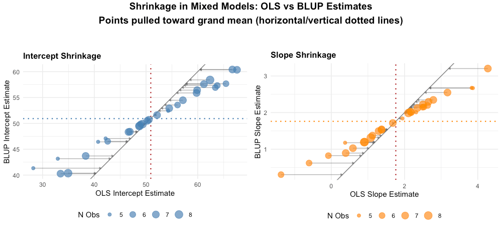
Suppose Person A has only 2 observations, both very high. If we estimate their trajectory independently (OLS), we'd get an extreme intercept based on just 2 points.
But we have information from 199 other people. Shouldn't that tell us something?
What Shrinkage Does
Mixed models "shrink" extreme individual estimates toward the group mean. The amount of shrinkage depends on:
- How extreme the person's data are: More extreme = more shrinkage
- How reliable the person's data are: Fewer observations = more shrinkage
- How variable the population is: Less population variability = more shrinkage
Three Approaches to Individual Estimation
| Approach | What it does | Limitation |
|---|---|---|
| Complete pooling | Everyone gets the grand mean | Misses real heterogeneity |
| No pooling (OLS) | Separate regression per person | Extreme estimates with sparse data |
| Partial pooling (LMM) | Weighted average of individual data and group mean | Best of both worlds |
LMM's partial pooling gives more weight to an individual's data when they have many observations and the data are consistent, and more weight to the group mean when observations are sparse or variable.
Why This Matters
- Better individual predictions: Shrunken estimates are typically more accurate than raw OLS estimates
- Handles sparse data: People with few observations still get reasonable estimates
- Automatic regularization: Protects against overfitting
Mathematical Foundations (optional formal notation)
The Two-Level Model
Level 1 (within-person):
yᵢₜ = β₀ᵢ + β₁ᵢ(Timeₜ) + εᵢₜ
Where εᵢₜ ~ N(0, σ²)
Level 2 (between-person):
β₀ᵢ = γ₀₀ + u₀ᵢ
β₁ᵢ = γ₁₀ + u₁ᵢ
Where the random effects follow a bivariate normal distribution:
[u₀ᵢ]     [0]   [τ₀₀  τ₀₁]
[u₁ᵢ] ~ N([0], [τ₁₀  τ₁₁])
(The random-effects covariance matrix is symmetric: τ₀₁ = τ₁₀.)
Combined Model
Substituting Level 2 into Level 1:
yᵢₜ = γ₀₀ + γ₁₀(Time) + u₀ᵢ + u₁ᵢ(Time) + εᵢₜ
Variance of Observations
The marginal variance of yᵢₜ at time t:
Var(yᵢₜ) = τ₀₀ + 2t·τ₀₁ + t²·τ₁₁ + σ²
The covariance between two observations from the same person at times t and t':
Cov(yᵢₜ, yᵢₜ') = τ₀₀ + (t + t')·τ₀₁ + (t × t')·τ₁₁
These expressions hold for any numeric time coding; centering time (e.g., at baseline or midpoint) improves interpretability and numerical stability.
Interactive Exploration
To build deeper intuition for how LMM parameters affect trajectories, use the interactive explorer below. Adjust the sliders to see how changing the intercept mean, slope variance, and other parameters affects the spaghetti plot in real-time.
This tool lets you:
- Adjust fixed effects (average intercept and slope) and see the mean trajectory change
- Modify random effect variances and watch individual trajectories spread out or converge
- Change the intercept-slope correlation to see fan-in or fan-out patterns
- Observe how the ICC changes as you adjust between- and within-person variance
Practical Considerations
Data Format
LMM requires long format: one row per observation.
Wide format (won't work):        Long format (required):

id   y_t1  y_t2  y_t3             id   time   y
1    48    52    56               1    0      48
2    55    54    57               1    1      52
                                  1    2      56
                                  2    0      55
                                  2    1      54
                                  ...
Missing Data
LMM handles missing observations gracefully:
- Uses all available outcome data under ML (observations can differ per person)
- Assumes MAR given the variables in the model; include auxiliary covariates when plausible
- Rows with missing predictors are typically dropped; consider imputation or modeling missingness
Caution: If dropout is related to the outcome trajectory itself (MNAR), estimates may be biased. Consider sensitivity analyses.
Intraclass Correlation (ICC)
The ICC tells you what proportion of total variance is between-person (stable individual differences) versus within-person (change + noise).
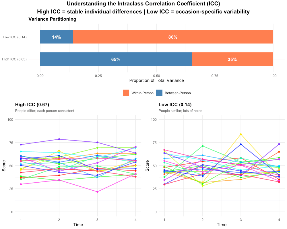
An ICC of 0.65 means 65% of variance is between persons—observations within a person are more similar to each other than to other people's observations. This justifies using mixed models: there's meaningful clustering to account for.
With random slopes, the ICC is time-dependent; the single-number ICC interpretation applies to random-intercept-only models.
Common Pitfalls
| Pitfall | Mistake | Fix |
|---|---|---|
| REML for fixed effects comparison | Comparing models with different fixed effects using REML | Use ML (REML = FALSE) for model comparison; REML likelihoods aren't comparable across fixed effects |
| Ignoring singular fit warnings | Dismissing "boundary (singular) fit" messages | A variance at zero means over-specification; check VarCorr() and simplify |
| Over-specifying random effects | Including random quadratic with only 4 time points | You need enough within-person observations for complex random effects; start simple |
| Treating BLUPs as data | Using extracted random effects in secondary analyses as observed data | BLUPs have uncertainty; include predictors in the model, not in post-hoc BLUP analyses |
| Time coded as factor | Treating time as categorical when you want a continuous slope | Factor time gives dummy variables, not a growth trajectory; use numeric time |
| Misinterpreting ICC | "ICC = 0.65 means the model explains 65%" | ICC is variance partitioning, not variance explained; it tells you between- vs. within-person split |
| Ignoring residual assumptions | Not checking normality and homoscedasticity of residuals | Severe violations bias SEs; plot residuals vs. fitted; consider AR(1) if closely spaced |
| Confusing marginal and conditional R² | Reporting only marginal R² when random effects matter | Marginal = fixed effects only; Conditional = fixed + random; report both |
| Conflating statistical and practical significance | "Slope variance is significant, so individual differences matter" | With large N, tiny variances are significant; interpret effect sizes substantively |
Summary
You now have the conceptual foundation for understanding LMM:
- Nested data require mixed models—ignoring the dependency structure produces misleading standard errors
- Fixed effects capture population-average trajectories; random effects capture individual variation around those averages
- Shrinkage improves individual estimates by borrowing strength across people—especially valuable with sparse data
- ICC tells you how much variance is between- vs. within-person, justifying the mixed model approach
This is enough to understand what LMM does and why. To actually fit one, continue to the worked example.
This overview covers two-level linear mixed models for continuous outcomes with a single clustering variable (persons). Not covered: three-level models (e.g., observations within persons within sites), generalized mixed models for binary/count outcomes (GLMM), Bayesian estimation (brms), nonlinear growth curves, and multivariate mixed models. See the tutorial links for code and estimation details.
Next Steps
Walkthrough: Worked Example → Step-by-step R code to simulate data, fit models, and interpret results.