When Outcomes Aren't Continuous
Many longitudinal outcomes aren't continuous — and they need models that respect their structure:
- Did the participant use a substance? (binary: yes/no)
- How many days did they use in the past month? (count: 0, 1, 2, …)
- What was their symptom severity rating? (ordinal: mild, moderate, severe)
Generalized Linear Mixed Models (GLMM) handle these outcomes by combining two ideas:
- Generalized linear models (GLM): Map the outcome to an appropriate scale through a link function, and model variance as a function of the mean
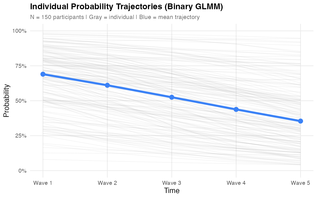
- Mixed models: Include random effects to capture individual-level variation over time
The result: individual trajectories for non-continuous outcomes, with proper handling of the outcome's distributional properties.
Treating these outcomes as continuous may seem harmless, but it creates real problems — predicted probabilities outside [0, 1], counts below zero, ordinal distances treated as equal. A model that predicts a -15% probability of substance use signals a fundamental mismatch between the model and the data's structure. GLMM avoids these issues by design.
Before reading further, consider your outcome variable:
- Type: Is it binary (yes/no), a count (0, 1, 2, …), or ordinal (mild/moderate/severe)?
- Boundaries: Does it have a floor at zero? Is it bounded between 0 and 1?
- Variance pattern: Does variability change with the level of the outcome?
These properties determine which distribution and link function your model needs. If your outcome is continuous, you likely need LMM instead.
What GLMM Provides
GLMM extends the LMM framework to handle the distributional properties of non-continuous outcomes:
Appropriate Outcome Modeling
Each outcome type gets a distribution that matches its properties — Bernoulli for binary, Poisson or negative binomial for counts, cumulative logit for ordinal. The model respects natural boundaries (probabilities between 0 and 1, counts ≥ 0) and correctly specifies how variance relates to the mean.
Individual Trajectories on the Latent Scale
Random effects operate on the link scale (e.g., log-odds for binary, log for counts), not the observed scale. Each person gets their own intercept and slope on this transformed scale, which then maps back to probabilities or expected counts through the inverse link function.
Conditional Interpretation
GLMM estimates are conditional — they describe the effect of a predictor for a specific individual, holding their random effects constant. This is the natural quantity when you care about within-person change: "How does this person's probability of substance use change over time?"
This contrasts with marginal (population-averaged) approaches like GEE, which answer: "How does the average probability change over time?" The distinction matters because averaging nonlinear functions gives different results than applying the function to averages.
Missing Data Handling
GLMM uses all available observations under maximum likelihood — participants who miss waves still contribute information without listwise deletion. The key assumption is Missing At Random (MAR): missingness can depend on observed variables, but not on the missing values themselves.
Handles Unbalanced Data Gracefully
Like LMM, GLMM naturally handles unbalanced designs — participants can have different numbers of observations, measurement timing can vary, and some waves can be missing entirely. You don't need complete data from everyone to fit the model.
Flexible Time Structures
Time can be equally spaced (0, 1, 2, 3, 4), unequally spaced (0, 3, 6, 12, 24 months), or person-specific (actual measurement dates). Code time as a continuous variable with appropriate values — the link function and random effects machinery work the same regardless of spacing.
Flexible Predictor Framework
Like LMM, you can include:
- Time-invariant predictors: Do males and females differ in their trajectories?
- Time-varying predictors: Does current stress predict this wave's outcome?
- Cross-level interactions: Does the effect of stress on the outcome differ across people?
When GLMM is Appropriate
GLMM works well when you have:
| Requirement | Guideline |
|---|---|
| Repeated measures | 3+ waves (fewer limits random effects structure) |
| Non-continuous outcome | Binary, count, ordinal, or proportions |
| Interest in individual differences | Not just average trends — person-level trajectories |
| Adequate sample | 50+ clusters minimum; 100+ recommended for complex models |
| Conditional effects needed | You want subject-specific (not population-averaged) estimates |
Key Components
The Link Function
The link function is what makes GLMM "generalized." It connects the linear predictor (the part that looks like a regression equation) to the expected value of the outcome:
g(μᵢₜ) = Xᵢₜβ + Zᵢₜbᵢ
Where g(·) is the link function, transforming the outcome's natural scale to one where linear modeling makes sense.
| Outcome | Distribution | Link | g(μ) | Inverse: μ = |
|---|---|---|---|---|
| Binary | Bernoulli | Logit | log(μ/(1-μ)) | 1/(1+e⁻ˣ) |
| Count | Poisson | Log | log(μ) | eˣ |
| Count (overdispersed) | Negative Binomial | Log | log(μ) | eˣ |
| Ordinal | Multinomial | Cumulative logit | log(P(Y≤k)/(1-P(Y≤k))) | — |
Why not just use a linear link? Consider a binary outcome. A linear model predicts:
P(y = 1) = β₀ + β₁·time
If β₀ = 0.8 and β₁ = 0.1, by Time 3 you predict P = 1.1. The logit link prevents this by mapping probabilities to the entire real line:
log(P/(1-P)) = β₀ + β₁·time
Now the linear predictor can take any value, and the inverse logit maps it back to [0, 1].
Random Effects Structure
Random effects in GLMM work the same way as in LMM — they capture individual deviations from population averages. The key difference is that these deviations operate on the link scale:
| Component | What It Captures |
|---|---|
| Random intercept | Person-specific baseline level (on link scale) |
| Random slope | Person-specific rate of change (on link scale) |
| Random effect variance | How much individuals differ |
| Random effect covariance | Relationship between starting level and change |
Critical insight: A random intercept in a logistic GLMM captures person-level variation in log-odds, not in probability. Two people with random intercepts of +1 and -1 differ by 2 units on the log-odds scale, but the probability difference depends on where they are on the curve — the logistic function is nonlinear, so the same log-odds difference produces different probability differences at different baseline levels.
Variance Structure
Unlike LMM where residual variance is a free parameter, GLMM outcome distributions have variance tied to the mean:
| Distribution | Variance |
|---|---|
| Bernoulli | μ(1-μ) — largest at p = 0.5 |
| Poisson | μ — variance equals the mean |
| Negative Binomial | μ + μ²/θ — allows overdispersion |
This mean-variance relationship is built into the model. You don't estimate a separate residual variance for binary or Poisson outcomes — it's determined by the distribution. When the data show more variance than the distribution implies (overdispersion), you need a distribution that accommodates it, such as the negative binomial for counts.
Mathematical Foundations (optional formal notation)
The GLMM Equation
For person i at time t:
Conditional model (given random effects):
g(μᵢₜ) = ηᵢₜ = x'ᵢₜβ + z'ᵢₜbᵢ
Where:
- g(·) = link function
- μᵢₜ = E(yᵢₜ | bᵢ) = conditional expected value
- x'ᵢₜβ = fixed effects (population-level)
- z'ᵢₜbᵢ = random effects (person-level deviations)
Distribution of random effects:
bᵢ ~ N(0, G)
Where G is the random effects covariance matrix:
     [σ²₀₀  σ₀₁]
G =  [σ₀₁   σ²₁₁]
For a random intercept and slope model:
- σ²₀₀ = variance of random intercepts
- σ²₁₁ = variance of random slopes
- σ₀₁ = covariance between intercepts and slopes
Conditional Distribution
yᵢₜ | bᵢ ~ f(μᵢₜ, φ)
Where f is the specified distribution (Bernoulli, Poisson, Negative Binomial) and φ is the dispersion parameter (if applicable).
Marginal Likelihood
The marginal likelihood integrates over the random effects:
L(β, G, φ) = ∏ᵢ ∫ [∏ₜ f(yᵢₜ | bᵢ, β, φ)] · g(bᵢ | G) dbᵢ
This integral generally has no closed-form solution, requiring numerical approximation (Laplace, adaptive Gauss-Hermite quadrature, or MCMC).
Interpretation
GLMM parameters live on the link scale. Interpretation requires transforming back to the natural scale — and understanding that these are conditional (subject-specific) effects.
Binary Outcomes (Logistic GLMM)
On the link scale, coefficients are log-odds. Exponentiate for odds ratios:
| Parameter | Link Scale | Natural Scale |
|---|---|---|
| Intercept | Log-odds at time = 0 | Probability = logit⁻¹(β₀) |
| Time coefficient | Change in log-odds per unit time | Odds ratio = exp(β₁) |
| Predictor coefficient | Difference in log-odds | Odds ratio = exp(β) |
Example: β₁ = -0.3 for time → OR = exp(-0.3) = 0.74. For a given individual, the odds of the outcome decrease by 26% per time unit.
Conditional vs. marginal: The OR from a GLMM is conditional — it applies to a specific person. The marginal OR (from GEE) is typically closer to 1.0 because averaging over heterogeneous individuals attenuates the effect. The more random effect variance, the larger this gap.
Count Outcomes (Log-link GLMM)
Coefficients are on the log scale. Exponentiate for incidence rate ratios (IRR):
| Parameter | Link Scale | Natural Scale |
|---|---|---|
| Intercept | Log expected count at time = 0 | Expected count = exp(β₀) |
| Time coefficient | Change in log count per unit time | IRR = exp(β₁) |
| Predictor coefficient | Difference in log count | IRR = exp(β) |
Example: β₁ = 0.15 for time → IRR = exp(0.15) = 1.16. For a given individual, the expected count increases by 16% per time unit.
Converting to Probability Scale (Binary)
For presentation, convert log-odds to predicted probabilities by applying the inverse logit function. Predictions at the "average" individual (random effects = 0) are conditional predictions at the random effect mean, not marginal (population-averaged) predictions — the distinction matters when random effect variance is large.
Conditional vs. Marginal: Why It Matters
This distinction is fundamental and often misunderstood. In a linear model, conditional and marginal effects are identical. In a GLMM, they aren't — because the link function is nonlinear.
Conditional (GLMM): "For a specific person, how does a one-unit increase in X change their log-odds?"
Marginal (GEE): "Across the population, how does a one-unit increase in X change the average probability?"
Conditional effects from GLMM:
  Person A (random intercept = -2): P changes from 0.12 → 0.18
  Person B (random intercept =  0): P changes from 0.50 → 0.62
  Person C (random intercept = +2): P changes from 0.88 → 0.93

Same log-odds change, different probability changes.

Population average (marginal): P changes from 0.50 → 0.58
Neither is "right" — they answer different questions. Use GLMM when individual-level effects matter. Use GEE when you want population-level summaries. See the GEE Overview for the marginal approach.
Interactive Exploration
To build deeper intuition for how GLMM parameters affect trajectories, use the interactive explorer below. Adjust the sliders to see how changing the intercept, slope, and random effect variances affects individual trajectories on both the response and link scales.
This tool lets you:
- Toggle between binary (logistic) and count (log-link) outcomes to see how different link functions shape trajectories
- Adjust fixed effects on the link scale and watch the response-scale trajectories change nonlinearly
- Modify random effect variances to see individual trajectories spread or converge
- Switch to link scale view to see the linear model underneath the nonlinear response
Practical Considerations
Estimation
Unlike LMM, GLMM doesn't have a closed-form solution — it uses numerical approximation to integrate over random effects. In practice you rarely need to worry about this, but it helps to know the options:
| Method | When to use | Trade-off |
|---|---|---|
| Laplace (default) | Most models | Fast; may lose accuracy with very few observations per person |
| AGQ (nAGQ = 7+) | Binary outcomes, < 5 obs/person | More accurate but slower; limited to simple random effect structures |
| Bayesian (MCMC) | Complex models, small samples | Most flexible; requires prior specification and convergence checks |
Practical guidance: Start with Laplace. For binary outcomes with few observations per person, compare with AGQ — if estimates change meaningfully, trust AGQ.
Overdispersion
Overdispersion means the data show more variance than the assumed distribution predicts. It's common with count data and doesn't apply to binary outcomes (Bernoulli variance is fully determined by the mean).
Detection: Compare the ratio of the Pearson residual deviance to residual degrees of freedom. Values substantially above 1.0 suggest overdispersion.
# Quick overdispersion check
overdisp_ratio <- sum(residuals(fit, type = "pearson")^2) / df.residual(fit)
Solutions:
- Switch from Poisson to negative binomial (adds a dispersion parameter)
- Add an observation-level random effect (OLRE) to a Poisson model
- Use quasi-Poisson (not available in mixed model packages; use NB instead)
Zero-Inflation
When count data have more zeros than the count distribution predicts, consider a zero-inflated model. This models two processes: (1) a binary process determining whether the count is structurally zero, and (2) a count process for non-structural zeros and positive counts.
# Zero-inflated negative binomial
fit_zi <- glmmTMB(count ~ time + (time | id),
                  zi = ~ 1,  # constant zero-inflation probability
                  family = nbinom2, data = df)
Test whether zero-inflation is needed by comparing AIC/BIC of the standard vs. zero-inflated model.
Convergence
GLMM convergence issues are more common than in LMM because of the nonlinear likelihood surface. Common strategies:
- Simplify random effects: Start with random intercept only; add random slopes if supported by the data
- Rescale predictors: Center continuous predictors and ensure time is on a reasonable scale
- Try different optimizers:
glmmTMBandlme4support multiple optimizers - Check for separation: In binary models, if a predictor perfectly predicts the outcome in some subgroup, the model can't converge
Sample Size Considerations
GLMM generally needs more data than LMM because:
- Information per observation is lower (binary outcomes carry less information than continuous)
- Estimation involves numerical integration
- Random slope models require sufficient within-person variation
Rules of thumb (binary outcomes):
- Random intercept only: 50+ clusters, 5+ observations per cluster
- Random intercept + slope: 100+ clusters, 5+ observations per cluster
- These are minimums — more is always better for stable estimates
Missing Data
GLMM uses all available observations under maximum likelihood — participants who miss waves still contribute information without listwise deletion. The key assumption is Missing At Random (MAR): missingness can depend on observed variables (e.g., treatment group, prior outcomes), but not on the unobserved missing values themselves.
- Include auxiliary covariates that predict missingness to make the MAR assumption more plausible
- Rows with missing predictors are typically dropped; consider imputation if predictor missingness is non-trivial
- Binary and count outcomes carry less information per observation than continuous outcomes, so missing data has a relatively larger impact on precision
Caution: If dropout is related to the outcome trajectory itself (MNAR — e.g., participants with worsening symptoms are more likely to leave the study), estimates may be biased. Consider sensitivity analyses or pattern-mixture models.
Common Pitfalls
| Pitfall | Mistake | Fix |
|---|---|---|
| Wrong-scale interpretation | Reporting β = −0.5 as "a decrease of 0.5" without specifying link scale | GLMM coefficients are log-odds or log; always state scale and provide OR/IRR |
| Treating conditional as marginal | Using GLMM ORs for population claims like "reduced prevalence by X%" | GLMM gives conditional (subject-specific) effects; use GEE or marginalize for population averages |
| Ignoring overdispersion | Fitting Poisson GLMM without checking variance > mean | Overdispersed Poisson gives too-small SEs; check and use negative binomial if needed |
| Over-specifying random effects | Adding random slopes for every predictor | Complex RE structures often fail to converge; start simple and let data guide complexity |
| Laplace vs. AGQ accuracy | Assuming Laplace approximation is always sufficient | For binary outcomes with < 5 observations per person, compare with nAGQ = 7; trust AGQ if they differ |
| Ignoring mean-variance relationship | Adding OLRE to a binary model "for overdispersion" | Bernoulli variance is determined by the mean; OLRE changes model meaning, not just variance |
| ORs without context | Reporting OR = 2.5 as "2.5 times more likely" | OR is odds ratio, not probability ratio; probability change depends on baseline |
| AIC across families | Comparing AIC between Poisson and NB from different packages | AIC is valid only for same data and same likelihood; use the same package for both |
| Ordinal as continuous | Treating a 4-point Likert scale as continuous in LMM | With < 5 categories, equal-interval assumption may distort results; use ordinal::clmm |
| No predicted probability plots | Interpreting only through ORs without plotting predictions | ORs are constant across range but probability changes are not; plot for practical significance |
Summary
GLMM extends the mixed model framework to handle outcomes that aren't continuous:
- Link functions transform the outcome scale so linear modeling applies — logit for binary, log for counts
- Random effects operate on the link scale, giving each person their own trajectory in log-odds or log-counts
- Conditional interpretation means effects are subject-specific — they describe what happens for a given individual, not the population average
- Variance is tied to the mean for most GLMM distributions — overdispersion and zero-inflation require explicit modeling
- Estimation is approximate — Laplace is fast but may be inaccurate for small clusters with binary outcomes; AGQ is more precise but slower
The conceptual leap from LMM to GLMM is smaller than it appears. If you understand random intercepts and slopes in a linear model, you understand them in a GLMM — they just live on a transformed scale.
This overview covers two-level GLMMs for binary and count outcomes with a single clustering variable (persons). Not covered: ordinal mixed models (ordinal::clmm), zero-inflated models in depth, Bayesian estimation (brms), spatial or crossed random effects, and multivariate GLMMs. See the tutorial links for code and estimation details.
Next Steps
Walkthrough: Worked Example → Step-by-step R code to simulate data, fit binary and count GLMMs, and interpret results.