When Your Focus Is the Population, Not the Person
Some longitudinal questions are about population-level patterns:
- Does this intervention reduce the average prevalence of substance use?
- Is the population rate of emergency visits declining over time?
- Across all participants, does the average count differ by treatment group?
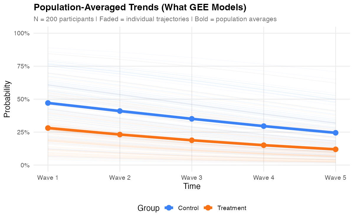
These are marginal questions — they ask what happens on average across the population. Answering them requires accounting for repeated measures on the same person, but it doesn't require modeling each person's individual trajectory.
Generalized Estimating Equations (GEE) are designed for exactly this. GEE takes a semi-parametric approach:
- Specify how the mean relates to predictors (the regression model)
- Specify a working correlation structure to approximate within-person dependence
- Use a sandwich estimator to produce valid standard errors even if the working correlation is wrong
The result: consistent, efficient estimates of population-averaged effects with robust inference and minimal distributional assumptions.
GEE and GLMM answer fundamentally different questions — neither is "better." If you need individual trajectories, random effect variances, or subject-specific predictions, see GLMM. If you need population-averaged effects with minimal distributional assumptions, read on.
What GEE Provides
Population-Averaged (Marginal) Effects
GEE estimates what happens to the average person in the population — not a specific individual. For binary outcomes, the coefficient describes how the population prevalence changes with a predictor. For counts, it describes how the population rate changes.
This distinction matters most for non-linear models. In a logistic GLMM, the odds ratio is conditional — it applies to a specific person holding their random effect constant. In GEE, the odds ratio is marginal — it describes the population-level association. The marginal OR is always closer to 1.0 than the conditional OR because averaging over heterogeneous individuals attenuates the effect.
Robust Standard Errors
GEE's signature feature is the sandwich (Huber-White) estimator. It produces valid standard errors and confidence intervals even when the working correlation structure is misspecified. This is a remarkable property: you can get the correlation structure wrong and still get valid inference for the regression coefficients.
The trade-off: if the working correlation is close to the truth, robust SEs are slightly less efficient than model-based (naive) SEs. If it's far from the truth, robust SEs protect you while naive SEs don't.
Minimal Distributional Assumptions
GEE doesn't require a full likelihood specification. You need:
- A correct mean model (how predictors relate to the outcome)
- A variance function (how variance relates to the mean)
- A working correlation structure (can be wrong — robust SEs cover you)
You do not need:
- A correctly specified random effects distribution
- The true correlation structure
- Normality of anything
This makes GEE particularly attractive when you distrust distributional assumptions or when the random effects distribution is genuinely non-normal.
Straightforward Interpretation
GEE coefficients have the same interpretation as coefficients from a standard GLM fit to independent data — just with appropriate standard errors for the correlation. No random effects to condition on, no link-scale complications for marginal summaries.
Handles Unbalanced Data Gracefully
Like LMM and GLMM, GEE naturally handles unbalanced designs — participants can have different numbers of observations, measurement timing can vary, and some waves can be missing entirely. The estimating equations use all available observations from each person.
Flexible Time Structures
Time can be equally spaced (0, 1, 2, 3, 4), unequally spaced (0, 3, 6, 12, 24 months), or person-specific (actual measurement dates). Code time as a continuous variable with appropriate values — the estimating equation machinery works the same regardless of spacing.
Missing Data: Important Limitation
Unlike LMM and GLMM (which handle MAR), standard GEE assumes Missing Completely At Random (MCAR) — the strongest and least realistic missing data assumption. If dropout depends on observed variables, GEE estimates may be biased without correction. See Practical Considerations for mitigations including weighted GEE and multiple imputation.
When GEE is Appropriate
| Requirement | Guideline |
|---|---|
| Repeated measures | 3+ waves (GEE works with 2, but limited) |
| Interest in population averages | Not individual trajectories |
| Adequate clusters | 40+ individuals minimum; 100+ recommended for robust SEs |
| Outcome type | Binary, count, ordinal |
| Missing data mechanism | MCAR or approximately MCAR (see below) |
Key Components
GEE has two distinctive building blocks beyond the mean model itself. Instead of specifying a full probability model (as GLMM does), GEE finds parameter values that make weighted residuals sum to zero across all participants — where the weights come from a working correlation structure and inference is protected by the sandwich estimator. See Mathematical Foundations for formal notation.
Working Correlation Structures
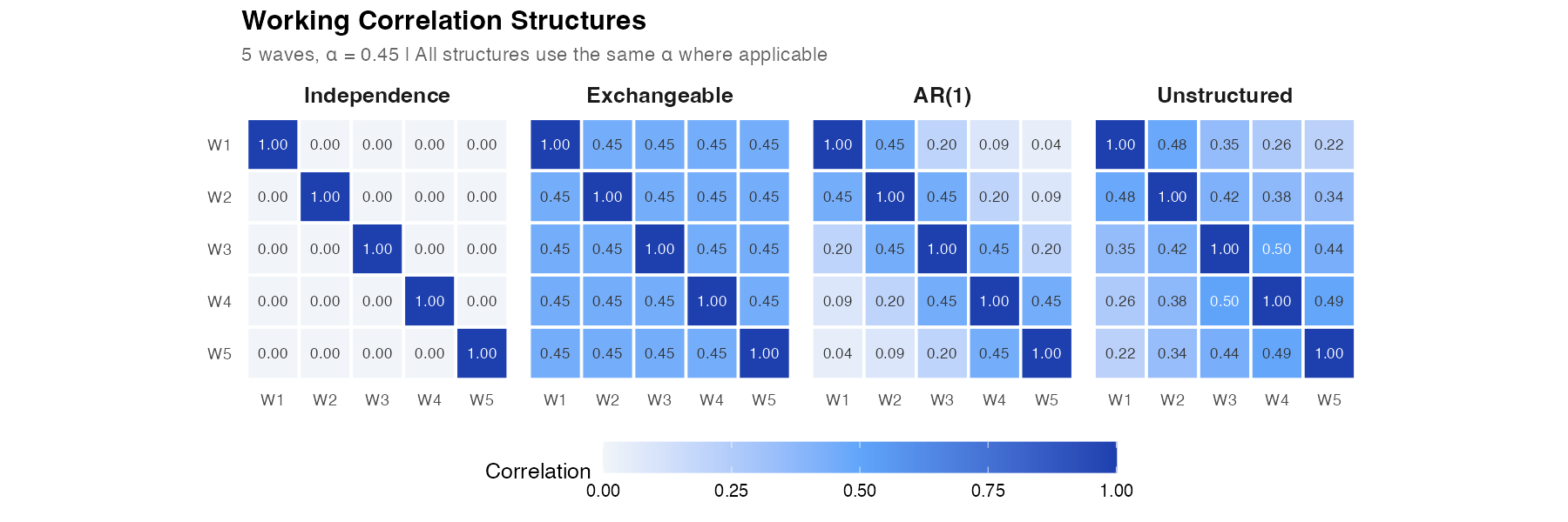
The working correlation matrix R(α) specifies how observations within a person are related. GEE offers several options:
| Structure | Pattern | Assumption | Parameters |
|---|---|---|---|
| Independence | All off-diagonals = 0 | No within-person correlation | 0 |
| Exchangeable | All pairs equally correlated | Compound symmetry | 1 (α) |
| AR(1) | Correlation decays with lag | Autoregressive | 1 (α) |
| Unstructured | Each pair has its own correlation | No pattern assumed | T(T−1)/2 |
With robust SEs, the choice of working correlation affects efficiency (precision) but not consistency (validity). A poorly specified working correlation gives wider confidence intervals than necessary, but they still have correct coverage. A close-to-correct working correlation gives tighter intervals.
The Sandwich Estimator
GEE's robustness comes from how it estimates the covariance of β̂:
Var(β̂) = B⁻¹ M B⁻¹
Where:
- B = model-based (naive) information matrix — what you'd get if the working correlation were correct
- M = "meat" — empirical correction based on observed residuals
The "bread-meat-bread" sandwich structure means:
- If the working correlation is correct: B⁻¹ M B⁻¹ ≈ B⁻¹ (sandwich ≈ naive)
- If the working correlation is wrong: B⁻¹ alone is invalid, but the sandwich correction fixes it
Small-sample adjustment: With fewer than 40–50 clusters, the sandwich estimator can underestimate standard errors. Use bias-corrected variants (e.g., sandwich = "MD" or sandwich = "KC" in some packages).
Mathematical Foundations (optional formal notation)
The GEE Framework
For person i with nᵢ observations, the marginal mean is:
g(μᵢₜ) = x'ᵢₜβ
Where g(·) is the link function (same choices as GLMM: logit, log, identity).
The marginal variance is:
Var(yᵢₜ) = φ · v(μᵢₜ)
Where v(·) is the variance function and φ is the dispersion parameter.
Estimating Equations
The GEE estimator β̂ solves:
U(β) = Σᵢ₌₁ᴺ D'ᵢ Vᵢ⁻¹ Sᵢ = 0
Where:
- Sᵢ = yᵢ − μᵢ(β) is the vector of residuals for person i
- Dᵢ = ∂μᵢ/∂β is the matrix of derivatives
- Vᵢ = φ Aᵢ^(1/2) R(α) Aᵢ^(1/2) is the working covariance
- Aᵢ = diag{v(μᵢ₁), …, v(μᵢₙᵢ)} contains variance function values
- R(α) is the working correlation matrix
Consistency
Under correct specification of the mean model E(yᵢₜ) = g⁻¹(x'ᵢₜβ), β̂_GEE is consistent for β regardless of the working correlation R(α).
Asymptotic Variance
√N(β̂ − β) → N(0, B⁻¹ M B⁻¹)
Where:
- B = Σᵢ D'ᵢ Vᵢ⁻¹ Dᵢ
- M = Σᵢ D'ᵢ Vᵢ⁻¹ Sᵢ S'ᵢ Vᵢ⁻¹ Dᵢ
This is the sandwich variance — valid under misspecification of R(α).
QIC (Quasi-likelihood Information Criterion)
QIC = -2Q(β̂ᵣ; I) + 2 trace(Ω̂ᵢ V̂ᵣ)
Where Q is the quasi-likelihood evaluated under independence working correlation, and the penalty adjusts for model complexity. Lower QIC = better fit.
Interpretation
GEE coefficients are marginal (population-averaged) effects on the link scale — the same scale as a standard GLM. This is GEE's interpretive advantage: no random effects to condition on.
Binary Outcomes (Logistic GEE)
Coefficients are log-odds of the population proportion. Exponentiate for marginal odds ratios:
| Parameter | Link Scale | Natural Scale |
|---|---|---|
| Intercept | Log-odds of population prevalence at time = 0 | Prevalence = logit⁻¹(β₀) |
| Time coefficient | Change in log-odds per unit time | Marginal OR = exp(β₁) |
| Predictor coefficient | Difference in log-odds | Marginal OR = exp(β) |
Example: β₁ = -0.25 for time → OR = exp(-0.25) = 0.78. Across the population, the odds of the outcome decrease by ~22% per wave.
Marginal vs. conditional: The marginal OR from GEE is always closer to 1.0 than the conditional OR from GLMM. This isn't bias — they answer different questions. The gap grows with random effect variance: more individual heterogeneity means more attenuation when averaging across individuals.
Count Outcomes (Log-link GEE)
Coefficients are on the log scale. Exponentiate for marginal incidence rate ratios (IRR):
| Parameter | Link Scale | Natural Scale |
|---|---|---|
| Intercept | Log population rate at time = 0 | Population rate = exp(β₀) |
| Time coefficient | Change in log rate per unit time | Marginal IRR = exp(β₁) |
| Predictor coefficient | Difference in log rate | Marginal IRR = exp(β) |
Example: β₁ = 0.10 for time → IRR = exp(0.10) = 1.11. Across the population, the expected rate increases by ~11% per wave.
Interactive Exploration
To build deeper intuition for how GEE works, use the interactive explorer below. Adjust the correlation structure and parameters to see how the working correlation matrix changes, how population-averaged (GEE) curves differ from conditional (GLMM) trajectories, and when robust SEs diverge from naive SEs.
This tool lets you:
- Switch correlation structures — see how Independence, Exchangeable, AR(1), and Unstructured produce different R(α) matrices for the same α
- Adjust α — watch the heatmap update in real-time as within-person correlation strengthens or weakens
- Compare marginal vs conditional — the bold red GEE curve shows the population average; faded lines show individual GLMM trajectories. Increase τ² to see the curves diverge
- Examine SE behavior — the bottom bar chart shows when robust SEs protect you from a misspecified working correlation (try Independence with high α)
Practical Considerations
Missing Data: The MCAR Requirement
GEE's most important limitation is its assumption about missing data:
| Mechanism | Definition | GEE Valid? |
|---|---|---|
| MCAR | Missingness is completely random — unrelated to any variables | Yes |
| MAR | Missingness depends on observed variables | Biased without correction |
| MNAR | Missingness depends on unobserved values | Biased |
Standard GEE assumes MCAR — the strongest and least realistic assumption. If participants who are getting worse are more likely to drop out (MAR), GEE estimates will be biased.
Mitigations for MAR dropout:
- Weighted GEE (WGEE): weight each observation by the inverse probability of being observed
- Multiple imputation + GEE: impute missing values, fit GEE to each imputed dataset, pool results
- Use GLMM instead — FIML/REML handles MAR naturally
Number of Clusters
The sandwich estimator is an asymptotic result — it works well with many clusters. With few clusters:
| Clusters | Recommendation |
|---|---|
| < 20 | Avoid GEE or use bias-corrected SEs with extreme caution |
| 20–40 | Use bias-corrected sandwich (Mancl-DeRouen or Kauermann-Carroll) |
| 40–100 | Standard sandwich is acceptable; bias-corrected is preferable |
| 100+ | Standard sandwich works well |
Choosing a Correlation Structure
In practice, the choice rarely matters much for point estimates (they're consistent regardless). It affects efficiency:
- Start with exchangeable — a safe default for most longitudinal data
- Compare with AR(1) if you expect temporal decay
- Use QIC (quasi-likelihood information criterion) to compare structures
- Check that robust and naive SEs are reasonably close — large discrepancies suggest the working correlation is far from reality
library(geepack)

fit_exch  <- geeglm(y ~ time + group, id = id, data = df,
                     family = binomial, corstr = "exchangeable")
fit_ar1   <- geeglm(y ~ time + group, id = id, data = df,
                     family = binomial, corstr = "ar1")
fit_indep <- geeglm(y ~ time + group, id = id, data = df,
                     family = binomial, corstr = "independence")
Common Pitfalls
| Pitfall | Mistake | Fix |
|---|---|---|
| Treating GEE coefficients as conditional | Interpreting GEE OR as applying to a specific person | GEE gives marginal (population-averaged) effects; marginal OR is always closer to 1.0 than conditional OR |
| Ignoring MCAR assumption with dropout | Using standard GEE when dropout is related to the outcome | If dropout is MAR, GEE is biased; use weighted GEE, multiple imputation, or GLMM with FIML |
| Using too few clusters | Fitting GEE with < 40 participants and trusting sandwich SEs | Sandwich estimator needs large N (clusters, not observations); use bias-corrected variants or GLMM |
| Over-interpreting working correlation | Reporting estimated α as the "true" within-person correlation | Working correlation is a nuisance parameter for efficiency, not a reliable correlation estimate |
| Comparing GEE and GLMM coefficients directly | Concluding one is wrong because ORs differ | They estimate different quantities; marginal OR < conditional OR by design |
| Using naive SEs instead of robust | Reporting model-based SEs without sandwich correction | Naive SEs require exactly correct working correlation; always report robust SEs |
| Unstructured correlation with many time points | Using corstr = "unstructured" with 10+ waves | Requires T(T−1)/2 parameters; becomes unstable with limited clusters; use exchangeable or AR(1) |
| Not checking robust vs. naive SE agreement | Never comparing the two SE sets | Large discrepancies (> 20%) signal misspecified working correlation; useful diagnostic |
| GEE for clustered data without thought | Using GEE for any clustering without considering cluster-level effects | GEE averages over clusters; if cluster variation matters substantively, use multilevel models |
| QIC as likelihood-based criterion | Using QIC as if it were AIC with the same properties | QIC is quasi-likelihood-based; useful for relative comparison within GEE, but not as theoretically grounded |
Summary
GEE provides population-averaged estimates for correlated data with minimal distributional assumptions:
- Marginal effects describe population averages — how the outcome changes across the population, not for a specific individual
- Working correlation structures approximate within-person dependence; the choice affects efficiency but not consistency
- Sandwich standard errors produce valid inference even when the working correlation is wrong — GEE's defining feature
- MCAR assumption is GEE's main limitation — informative dropout biases estimates without correction
- Fewer assumptions than GLMM — no random effects distribution required — but also fewer capabilities (no individual predictions, no variance components)
The choice between GEE and GLMM isn't about which is "better" — it's about which question you're asking. Use GEE when the population average is the quantity of interest and you want robust, assumption-light inference.
This overview covers standard GEE for binary and count outcomes with a single clustering variable (persons). Not covered: weighted GEE for MAR dropout, ordinal GEE (see Reference for ordgee syntax), multinomial GEE (multgee), penalized GEE, doubly robust estimators, and alternating logistic regressions.
Next Steps
Walkthrough: Worked Example → Step-by-step R code to fit GEE models, compare correlation structures, and examine robust SEs.