Overview

Big Linear Mixed Models (BLMM) is a Python toolbox designed for fitting mass-univariate linear mixed models at scale—an approach especially well-suited for neuroimaging applications involving large cohorts and high-dimensional surface or voxelwise outcomes. In this tutorial, we walk through how to understand and interpret BLMM outputs using results derived from ABCD Study® neuroimaging data. The analyses featured here come from two mass-univariate linear mixed models applied to cortical surface data collected during the ABCD working-memory N-back task. In this experiment, the response variable of interest was the percent BOLD (Blood Oxygenation Level Dependent) signal, examined across thousands of brain locations. In this example we focus on interpreting the BLMM results, examining what the BLMM toolbox produces, how to read its statistical outputs, and how to draw clear scientific conclusions from them.

Stats

Subjects:5,179

Observations:9,835

Fixed Effects:23

Contrasts Tested:5

Random Effects:Subject-level intercepts and slopes

When to Use:

Large-scale longitudinal neuroimaging analyses with repeated measures, where traditional mixed model software struggles with computational demands

Key Advantage:

Scales to tens of thousands of images with vertex/voxel-wise analysis while properly accounting for within-subject correlation

What You'll Learn:

How to interpret BLMM output files including fixed effects (β), variance components (σ², D), t-statistics, and p-values mapped onto cortical surfaces

Data Access

Study Background

The data presented in this tutorial are drawn from the Adolescent Brain Cognitive Development (ABCD) Study, the largest long-term study of brain development and child health in the United States. The ABCD Study follows approximately 12,000 youth from age 9-10 through early adulthood, collecting neuroimaging, behavioral, and environmental data at regular intervals.

Task and Response Variable

The experiment conducted in this study was a working memory N-back task. The response variable of interest was the percent BOLD (Blood Oxygenation Level Dependent) signal—a measure of blood flow in the brain which acts as a proxy for neuronal activity.

Prior analyses produced a 2-vs-0 back contrast image for each subject and session, reflecting the subject's average percent BOLD change in response to the 2-back task during a particular session. In each image, the average percent BOLD change is recorded for every vertex on a predefined cortical surface.

Sample Characteristics

In total, the response data consists of 9,835 fMRI surface images. These images were drawn from 5,179 subjects, each of whom had data recorded for between 1 and 3 visits.

Viewer Data

The pre-processed BLMM results used by the interactive viewer are available in the public/data/blmm/ directory. This includes:

Surface geometry: FreeSurfer fsaverage5 pial surfaces (10,242 vertices per hemisphere)
Statistics: T-statistics, -log₁₀(p-values), beta coefficients, and residual variance for each contrast
Metadata: JSON files describing volume labels, colormaps, and suggested thresholds

These files represent aggregated vertex-wise statistics derived from the BLMM analysis—not the original subject-level fMRI images, which remain under ABCD data use agreements.

Design Matrix

We are interested in understanding how a range of independent variables impacted the task-specific percent BOLD response. The design matrix for both analyses included:

Intercept: Modeling average response
Sex: The subject's biological sex
Cross-sectional Age: The age of the subject at the first timepoint
Longitudinal Time: The difference in the subject's age from the first timepoint recorded
NIH Cognition Score (Age Corrected): The subject's age-corrected total score from the neurocognitive battery derived from seven measures from the NIH Toolbox
Race: Categorical variable indicating the subject's race (white, black, asian, or other)
Ethnicity: Categorical variable indicating the subject's ethnicity (hispanic or other)
Parental Education Level: Categorical variable representing the subject's parent's education (high school, college, bachelor, postgraduate)
Family Income: Categorical variable representing the subject's family income (less than 50K, 50K-100K, greater than 100K)
Marital Status: Categorical variable representing the marital status of the subject's parents

Data Preparation

The Linear Mixed Model

The Linear Mixed Model can be represented in the form:

Y = X\beta + Zb + \epsilon, \quad \epsilon \sim N(0,\sigma^2I), \quad b \sim N(0,\sigma^2D)

where, assuming the model includes $n$ observations, $p$ fixed effects and $q$ random effects, the model matrices are:

$X$ : the $(n \times p)$ fixed effects (independent variables) design matrix
$Z$ : the $(n \times q)$ random effects design matrix

The random terms are:

$Y$ : the $(n \times 1)$ response vector
$\epsilon$ : the $(n \times 1)$ error vector
$b$ : the $(q \times 1)$ random effects vector

Our interest lies in estimating the parameters:

$\beta$ : the $(p \times 1)$ fixed effects coefficient vector
$\sigma^2$ : the scalar residual variance
$D$ : the $(q \times q)$ random effects covariance matrix

The input and output of BLMM is labeled according to these notational conventions.

Analysis Designs

The two analysis designs differed in the random effects included in the model:

Design 1: Included a subject-level intercept as a random effect. This models the within-subject variability in the data.
Design 2: Included both a subject-level intercept and longitudinal time effect. This models the variation in individual subject's trajectories.

As random slopes cannot be considered for singleton subjects (those with only one observation), Design 2 was constrained to consider only subjects with 2 or more visits.

BLMM Configuration

# Example blmm_inputs.yml structure
Missingness:
  MinPercent: 0.5
X: /path/to/X.csv
Y_files: /path/to/y_files.txt
analysis_mask: /path/to/analysis/mask
clusterType: SLURM
Z:
- f1:
    design: /path/to/factor_design_matrix.csv
    factor: /path/to/factor_vector.csv
contrasts:
- c1:
    name: Intercept
    vector: [1, 0, 0, 0, 0, 0, 0, 0, 0, 0, 0, 0, 0, 0, 0, 0, 0, 0, 0, 0, 0, 0, 0]
- c2:
    name: Sex
    vector: [0, 1, 0, 0, 0, 0, 0, 0, 0, 0, 0, 0, 0, 0, 0, 0, 0, 0, 0, 0, 0, 0, 0]
- c3:
    name: CrossSectionalAge
    vector: [0, 0, 1, 0, 0, 0, 0, 0, 0, 0, 0, 0, 0, 0, 0, 0, 0, 0, 0, 0, 0, 0, 0]
- c4:
    name: LongitudinalTime
    vector: [0, 0, 0, 1, 0, 0, 0, 0, 0, 0, 0, 0, 0, 0, 0, 0, 0, 0, 0, 0, 0, 0, 0]
- c5:
    name: NIHScore
    vector: [0, 0, 0, 0, 1, 0, 0, 0, 0, 0, 0, 0, 0, 0, 0, 0, 0, 0, 0, 0, 0, 0, 0]
outdir: /path/to/output

Configuration Explanation

In the configuration file:

Missingness: The MinPercent: 0.5 parameter tells BLMM to report results for any vertex with at least 50% of observations present
X.csv: Contains the fixed effects design matrix of size $(n \times p)$
Y_files.txt: A text file containing paths to the surface images
analysis_mask: Specifies which vertices to analyze
clusterType: The type of computational cluster (e.g., Local, SLURM, SGE)
Z: Specifies random effects structure. The factor file is an $(n \times 1)$ vector indicating which subject each observation belongs to. The design file contains the random effects design matrix.
contrasts: Defines the null hypotheses to test (here: Intercept, Sex, Age, Time, NIH Score)

Statistical Analysis

Loading Libraries

import os
import numpy as np
import nibabel as nib
from demo.plot import plot_brain_surface

# Geometry file paths (FreeSurfer pial surfaces)
geom_lh = "demo/geom/lh.pial"
geom_rh = "demo/geom/rh.pial"

Output File Structure

BLMM produces the following output files for each analysis:

File	Description	Dimensions
`blmm_vox_beta.dat`	Fixed effect estimates (β)	vertices × 23 coefficients
`blmm_vox_con.dat`	Contrast estimates	vertices × 5 contrasts
`blmm_vox_conSE.dat`	Standard errors for contrasts	vertices × 5 contrasts
`blmm_vox_conT.dat`	T-statistics for contrasts	vertices × 5 contrasts
`blmm_vox_conTlp.dat`	-log₁₀(p-values)	vertices × 5 contrasts
`blmm_vox_sigma2.dat`	Residual variance (σ²)	vertices × 1
`blmm_vox_D.dat`	Random effects covariance (D)	vertices × elements of D
`blmm_vox_n.dat`	Sample size per vertex	vertices × 1
`blmm_vox_llh.dat`	Log-likelihood	vertices × 1
`blmm_vox_edf.dat`	Effective degrees of freedom	vertices × 1

Results are organized by hemisphere (lh/rh) and design (des1/des2).

Viewing Results

# Specify the analysis to examine
analysis = "des1"  # or "des2" for random slopes model
hemisphere = "lh"  # or "rh"

# Load t-statistics for contrasts
data_path = f"demo/results_{hemisphere}_{analysis}/blmm_vox_conT.dat"

# Visualize a specific contrast (volume_number selects the contrast)
# Volume 0 = Intercept, 1 = Sex, 2 = Age, 3 = Time, 4 = NIH Score
plot_brain_surface(data_path, geom_lh, volume_number=1)

Interactive Viewer

Use the interactive viewer below to explore BLMM outputs across designs, contrasts, and statistics. Start with Design 1 and the conT statistic, then adjust the contrast volume and threshold to see how patterns shift across the cortex.

Interpretation of T-Statistics

In the viewer, set Design 1, Statistic = conT, and Volume = 1 (Sex). Key observations:

Color scale: Blue indicates negative effects, red indicates positive effects
Threshold: Values with |t| < 2.0 are shown in gray (approximately p > 0.05)
Spatial patterns: Strong bilateral effects are visible in frontal and parietal regions associated with working memory

Understanding Different Output Types

To compare BLMM outputs, keep the same design and contrast, then switch the statistic in the viewer:

beta (β): Raw fixed effect coefficients. Values represent the estimated change in percent BOLD per unit change in the predictor.
conT: T-statistics for testing whether contrasts differ from zero. Larger absolute values indicate stronger evidence against the null hypothesis.
conTlp: Negative log₁₀ of p-values. Values > 1.3 correspond to p < 0.05; values > 2 correspond to p < 0.01. This transformation makes significant regions more visually apparent.
sigma2 (σ²): Residual variance at each vertex. Higher values indicate more unexplained variability in the BOLD response.

Contrast Interpretation

Use the viewer to step through the five contrasts (Volume 0–4) and compare spatial patterns:

Volume 0 (Intercept): Average BOLD response during the 2-back task
Volume 1 (Sex): Difference in BOLD response between males and females
Volume 2 (Cross-sectional Age): Association between baseline age and BOLD response
Volume 3 (Longitudinal Time): Change in BOLD response over time within individuals
Volume 4 (NIH Score): Association between cognitive performance and BOLD response

Each contrast reveals distinct spatial patterns, reflecting the neural correlates of these demographic and cognitive factors.

Static Reference Images

Can't access the interactive viewer? Click to view static visualizations

The images below show key BLMM outputs for reference. These are static versions of what the interactive viewer displays.

T-Statistics Overview (Both Hemispheres)

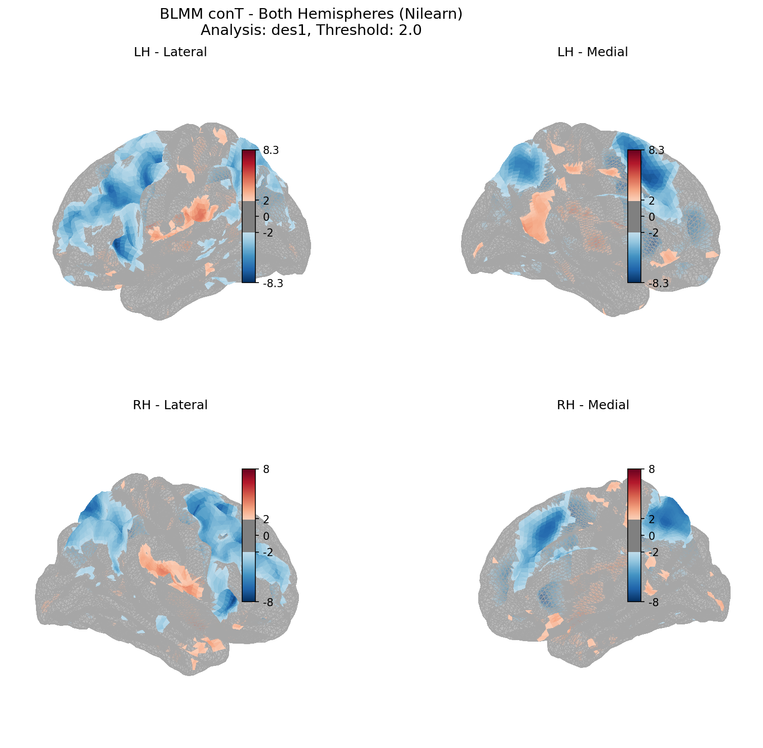
BLMM T-statistics for both hemispheres showing Design 1 results with threshold of 2.0

T-statistics from Design 1 (random intercepts only) mapped onto both cortical hemispheres. Blue indicates negative effects, red indicates positive effects. Values with |t| < 2.0 are shown in gray.

Statistics Comparison

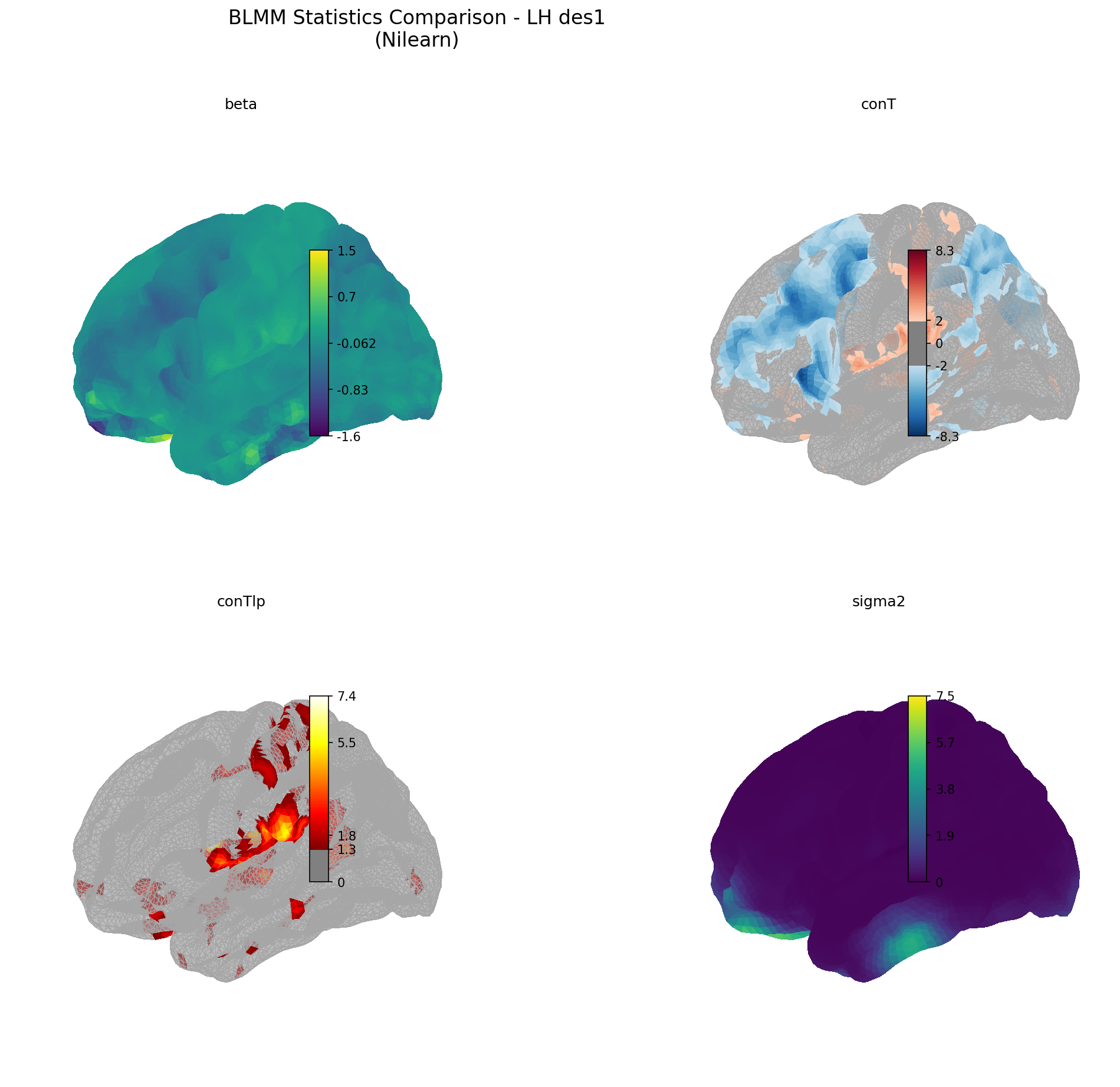
Comparison of different BLMM output statistics: beta coefficients, t-statistics, -log10(p-values), and residual variance

Four key output types from BLMM: beta coefficients (β), t-statistics (conT), negative log₁₀ p-values (conTlp), and residual variance (σ²). Each reveals different aspects of the analysis results.

All Contrasts Overview

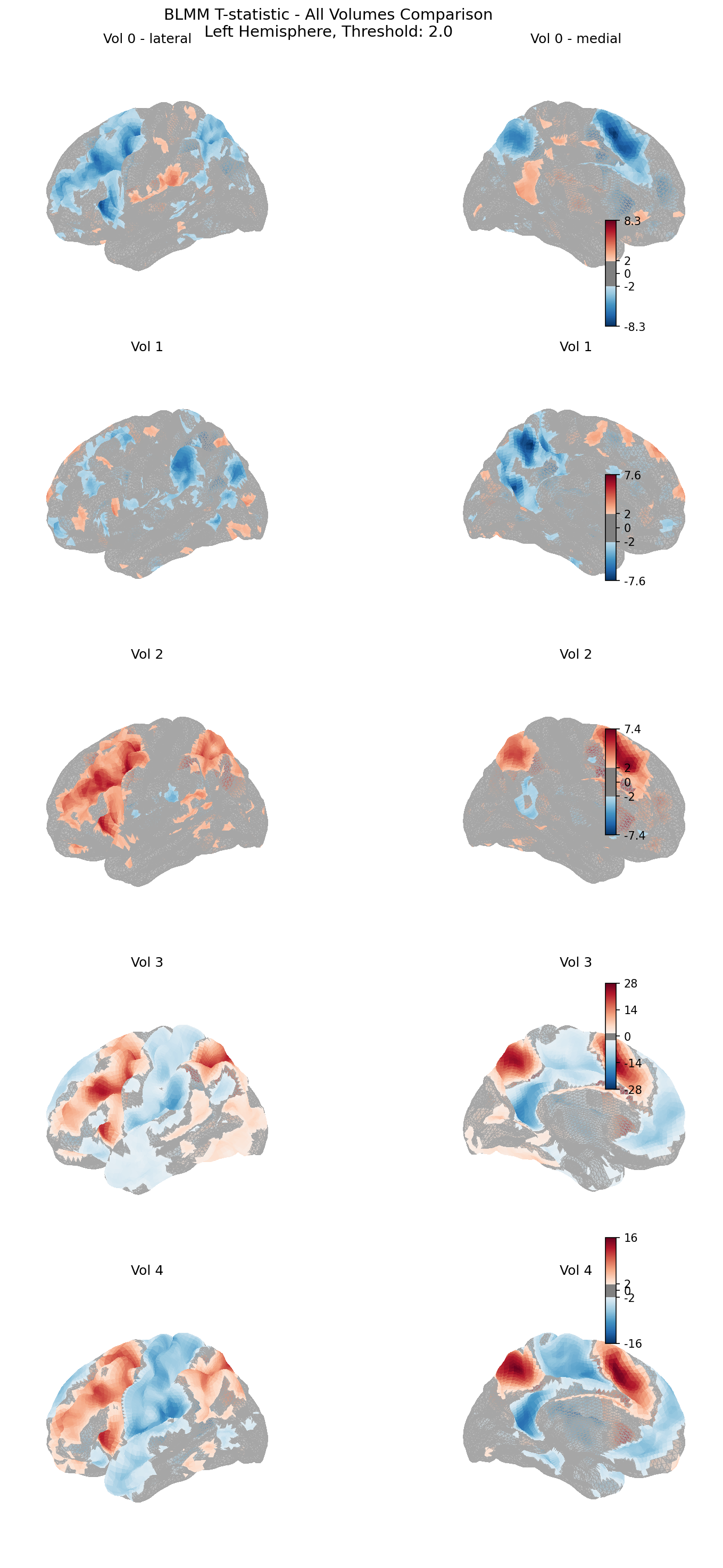
Overview of all five contrast t-statistics across left hemisphere

T-statistics for all five contrasts (Intercept, Sex, Cross-sectional Age, Longitudinal Time, NIH Score) displayed on the left hemisphere.

Discussion

Model Comparison

BLMM allows for formal comparison between nested models using likelihood ratio tests. In this example, we compared:

Design 1: Random intercepts only (simpler model)
Design 2: Random intercepts + random slopes for time (more complex model)

The comparison tests whether allowing individual trajectories to vary significantly improves model fit. This is implemented via the blmm_compare function, which outputs chi-squared statistics at each vertex.

Important: To perform comparison, the analyses must have equal sample sizes. The comparison shown is between Design 2 and a reduced version of Design 1 containing only subjects with 2 or more visits.

When to Choose Each Design

Design 1 (Random Intercepts) is appropriate when:

You have many singleton subjects (single timepoint)
Primary interest is in between-subject effects
Computational resources are limited

Design 2 (Random Intercepts + Slopes) is appropriate when:

Most subjects have multiple timepoints
Individual trajectories are expected to vary
You want to model heterogeneity in longitudinal change

Interpreting Results

When interpreting BLMM results:

Multiple comparisons: With thousands of vertices tested, appropriate correction for multiple comparisons is essential (e.g., FDR, permutation testing)
Effect sizes: T-statistics indicate statistical significance but not practical importance. Consider the magnitude of β coefficients.
Spatial coherence: Isolated significant vertices may be noise; look for spatially coherent clusters

Limitations

BLMM assumes normally distributed residuals; violations may affect inference
The mass-univariate approach treats each vertex independently, ignoring spatial correlation

Additional Resources

BLMM GitHub Repository

CODE

The official BLMM repository contains installation instructions, documentation, and example configurations for running your own analyses.

Visit Resource

BLMM NeuroImage Paper

PAPER

The methodology paper describing the BLMM algorithm, validation studies, and computational approach.

Visit Resource

ABCD Study

DATA

The Adolescent Brain Cognitive Development Study website with information about data access and study protocols.

Visit Resource

FreeSurfer

TOOL

FreeSurfer is used for cortical surface reconstruction and provides the geometry files used in BLMM surface analyses.

Visit Resource

Nilearn

DOCS

Python library for neuroimaging data analysis and visualization, useful for exploring BLMM outputs.

Visit Resource