Why Study Growth?
Longitudinal data capture something powerful: change. When you measure the same people over time, you can ask questions that matter:
- How do symptoms evolve after treatment begins?
- Do children's reading skills develop at the same rate?
- Does cognitive decline accelerate with age?
These are questions about trajectories—not just whether groups differ at a single moment, but how individuals change over time.
Traditional approaches like repeated measures ANOVA focus on group means: "Did the average score increase?" But that question often misses what we actually care about.
Consider a therapy study where the average patient improves by 8 points over 6 months. Success? Look at the individual trajectories:
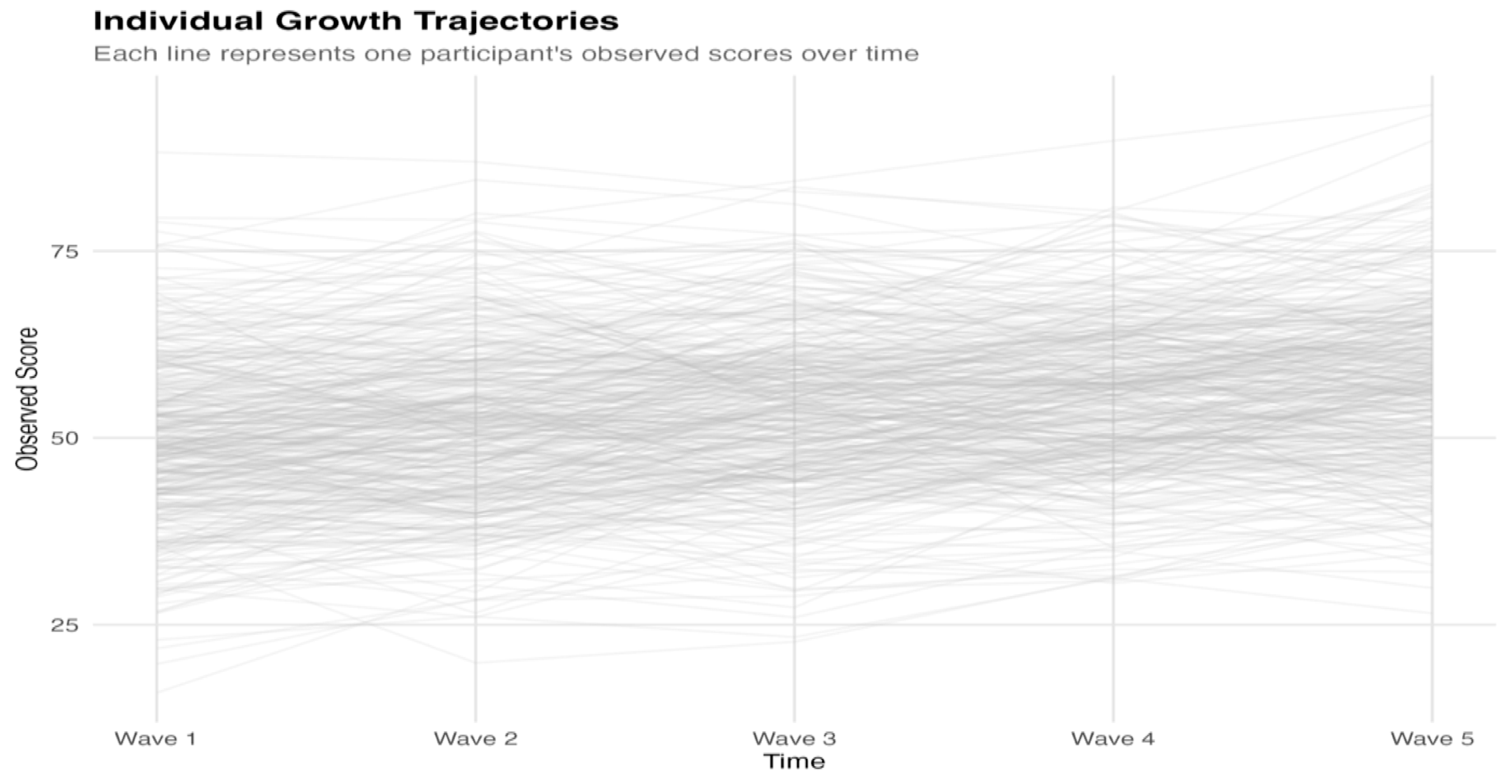
The average tells you "the group improved"—but the real questions are:
- How much do people differ in their starting points?
- How much do they differ in their rates of change?
- Are these two things related? (Do high starters change faster or slower?)
Latent Growth Curve Models (LGCM) answer exactly these questions. Every person gets their own trajectory—a starting point (intercept) and rate of change (slope)—and the model quantifies how much people vary in these trajectories.
Look at the spaghetti plot above. Before reading further, consider:
- Intercept variance: How spread out are the starting points at Wave 1?
- Slope variance: Do the lines fan out over time, or stay roughly parallel?
- Intercept-slope relationship: Do high starters tend to change faster, slower, or neither?
Hold these observations in mind—we'll return to them when discussing the model parameters.
What LGCM Provides
LGCM offers four capabilities that simpler methods lack:
Individual Trajectories
Each person has their own growth curve. The model estimates not just the average trajectory, but the variance around it—how much people differ in starting points and rates of change.
Flexible Time Structures
Waves don't need to be equally spaced. Measure at baseline, 3 months, 6 months, and 2 years? No problem—just code time accordingly. The slope becomes "change per unit time" in whatever metric you choose.
Missing Data Handling
Modern estimation (Full Information Maximum Likelihood) uses all available data. Participants who miss a wave still contribute information—no listwise deletion required.
Testable Model Fit
Unlike approaches that simply estimate parameters, LGCM produces fit indices. You can ask: Does a linear trajectory actually describe these data? Is a more complex model (quadratic, piecewise) warranted?
When LGCM is Appropriate
LGCM works well when you have:
| Requirement | Guideline |
|---|---|
| Repeated measures | 3+ waves (4+ preferred for testable fit) |
| Outcome type | Continuous (or ordinal; prefer categorical estimators such as WLSMV; 5+ categories often treated as approximately continuous—verify robustness) |
| Interest in individual differences | Not just "did the mean change?" |
| Adequate sample | 100+ for simple models; more for complex |
Key Components
Regardless of your statistical background, these are the building blocks of every LGCM.
The Two Latent Factors
Every person in your study has two numbers you can't directly observe:
| Factor | What It Captures | Defined By |
|---|---|---|
| Intercept (η₁) | Each person's level at Time = 0 | Where you place "0" in time coding |
| Slope (η₂) | Each person's rate of change per time unit | Constant in linear model |
These aren't measured directly—LGCM infers them from the pattern of observed scores across time.
Extensions: Add time-varying covariates (TVCs) to predict the outcome at each occasion, and time-invariant covariates (TICs) to predict the latent intercept and slope. TVCs capture occasion-specific influences; TICs capture stable between-person differences.
A useful analogy: In traditional factor analysis, multiple items measure one latent construct. In LGCM, multiple time points measure two latent constructs—where you start and how you change. The key difference is that LGCM's factor loadings aren't estimated from data; they're fixed to encode your time structure.
Factor Loadings: Encoding Time
In the linear LGCM presented here, slope loadings are fixed to encode time (0, 1, 2, …). Variants like latent-basis or piecewise growth free or re-fix some loadings to capture nonlinearity.
| Factor | Loadings | Why |
|---|---|---|
| Intercept | 1, 1, 1, 1, 1 | Contributes equally at every time point |
| Slope | 0, 1, 2, 3, 4 | Encodes time; contribution grows linearly |
The loadings 0, 1, 2, 3, 4 assume equally spaced waves with Time 0 at Wave 1. See Time Coding for centering options and unequal spacing.
Factor Means: The Average Trajectory
| Parameter | Symbol | Interpretation |
|---|---|---|
| Intercept mean | μ₁ | Average starting level across people |
| Slope mean | μ₂ | Average rate of change across people |
Together they define the average trajectory:
Average score at time t = μ₁ + μ₂ × t
Example: If μ₁ = 50 and μ₂ = 2, the average person starts at 50 and increases by 2 per wave.
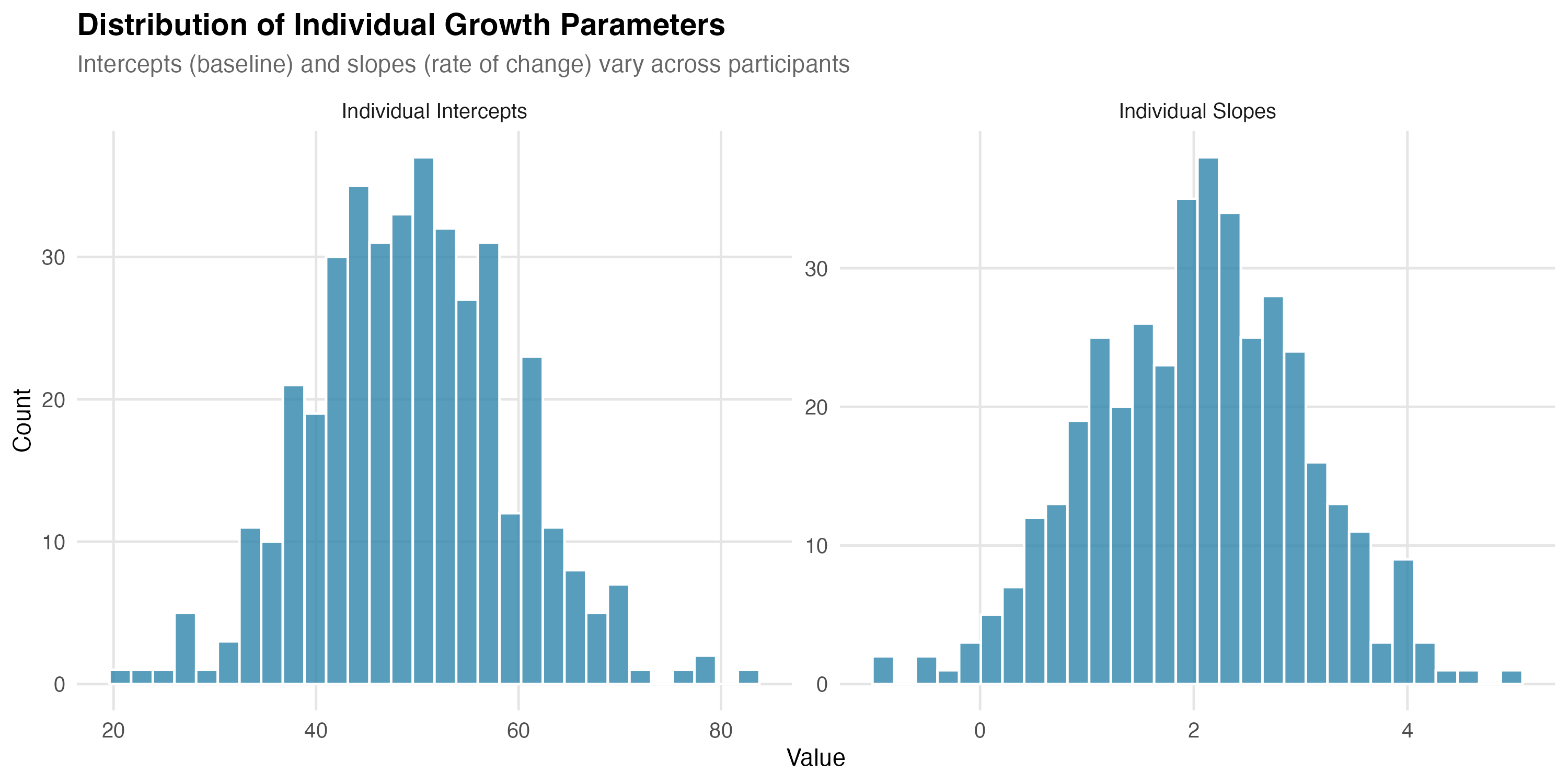
Factor Variances: Individual Differences
This is where LGCM shines—quantifying how much people differ.
| Parameter | Symbol | Interpretation |
|---|---|---|
| Intercept variance | ψ₁₁ | How much people differ in starting levels |
| Slope variance | ψ₂₂ | How much people differ in change rates |

Left: Low slope variance—everyone changes at similar rates, so lines stay roughly parallel. Right: High slope variance—some people improve rapidly, others stay flat, some decline. The dark line represents the mean trajectory in both cases.
Interpreting scale: Variances are in squared units. Take the square root for the standard deviation:
- If ψ₁₁ = 100 → SD = 10 → ~68% of people have intercepts within ±10 of the mean
- If ψ₂₂ = 1 → SD = 1 → ~68% of people have slopes within ±1 of the mean
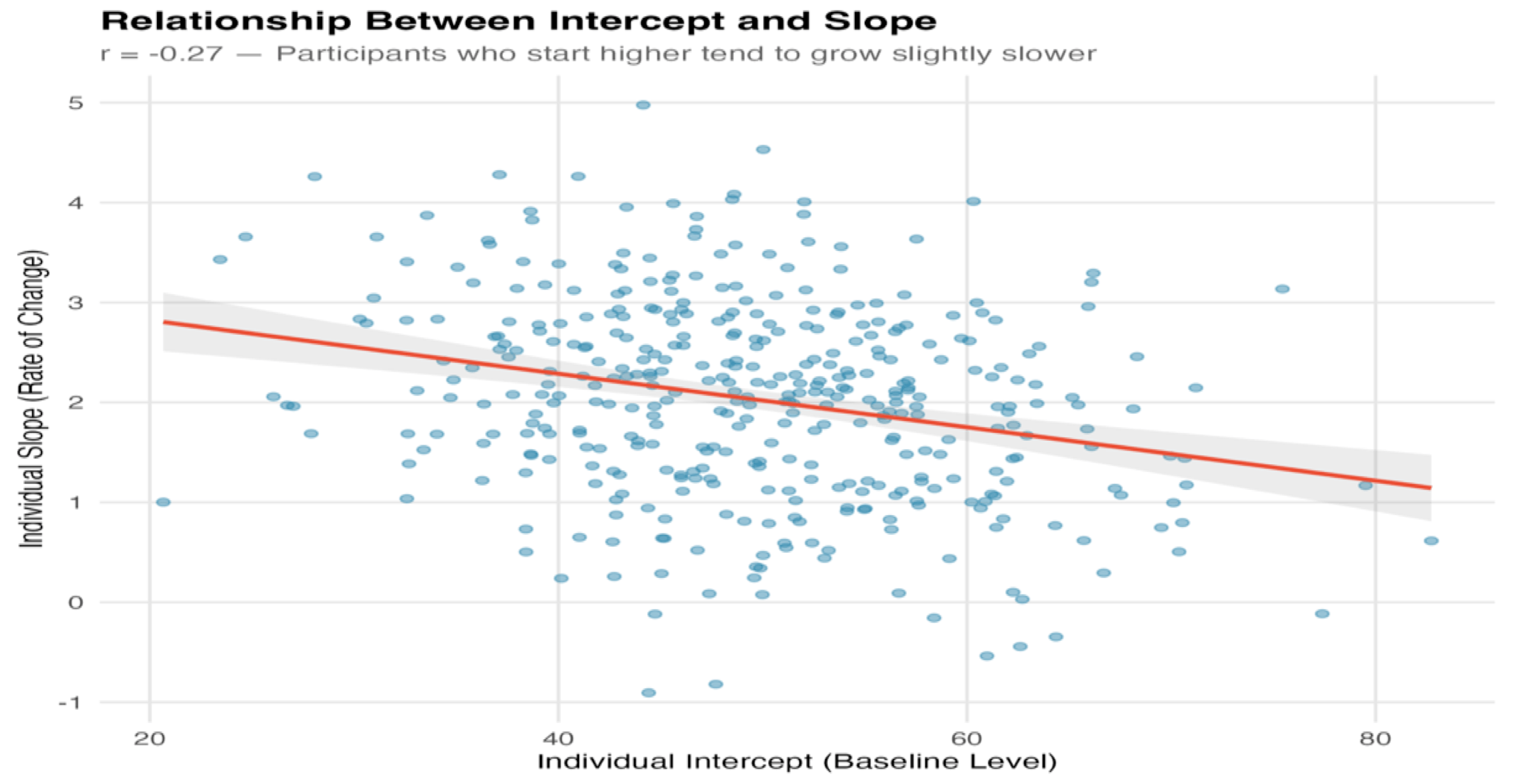
Factor Covariance: The Intercept-Slope Relationship
One of LGCM's most informative parameters is the relationship between where people start and how fast they change:
| Sign | Interpretation |
|---|---|
| Positive | High starters grow faster (or decline slower). "Rich get richer." |
| Negative | High starters grow slower (or decline faster). Catching up or ceiling effects. |
| Zero | Starting level doesn't predict change rate. |
These patterns have substantive meaning:
- A negative intercept-slope correlation in a therapy study might mean patients with severe symptoms improve more
- A positive correlation in educational research might indicate a "Matthew effect" where initial advantages compound over time
Convert covariance to correlation for easier interpretation:
r = ψ₁₂ / √(ψ₁₁ × ψ₂₂)
A correlation of -0.20 means a modest negative relationship: those who start higher grow slightly slower.
If the slope variance (ψ₂₂) is very small or near a boundary, the intercept–slope covariance/correlation can be unstable; inspect confidence intervals and consider rescaling time or centering to improve estimation.
Residuals: What the Trajectory Doesn't Explain
Observed = Predicted + Residual
yᵢₜ = (η₁ᵢ + η₂ᵢ × t) + εᵢₜ
Residual variance (θ) captures the noise around individual trajectories—measurement error, occasion-specific factors, or model misspecification.
Key assumptions:
- Residuals uncorrelated across time (can be relaxed in advanced models)
- Can be equal or freely estimated across waves
Mathematical Foundations (optional formal notation)
The Individual Trajectory Equation
Each person's score at time t follows:
yᵢₜ = η₁ᵢ + η₂ᵢ × λₜ + εᵢₜ
Where:
- yᵢₜ = observed score for person i at time t
- η₁ᵢ = person i's intercept (latent)
- η₂ᵢ = person i's slope (latent)
- λₜ = time coding for occasion t (fixed: 0, 1, 2, 3, 4)
- εᵢₜ = residual (measurement error + occasion-specific variation)
Distribution of Growth Factors
The intercept and slope follow a bivariate normal distribution:
[η₁]     [μ₁]   [ψ₁₁  ψ₁₂]
[η₂] ~ N([μ₂], [ψ₁₂  ψ₂₂])
This means:
- μ₁, μ₂ = population means (the "average" trajectory)
- ψ₁₁, ψ₂₂ = variances (individual differences in intercept and slope)
- ψ₁₂ = covariance (relationship between starting level and change)
For identification, observed item/indicator intercepts are fixed to 0, and we estimate the latent factor means; the latent intercept mean is thus the expected score at time = 0 (given the chosen time coding).
Model-Implied Covariance Structure
LGCM is a structural equation model. It implies a specific covariance matrix:
Σ = ΛΨΛ' + Θ
Where:
- Λ = factor loading matrix (fixed time codes)
- Ψ = factor covariance matrix (estimated)
- Θ = residual covariance matrix (typically diagonal)
Model fit tests whether your observed covariance matrix matches this implied structure.
Degrees of Freedom
| Components | Count |
|---|---|
| Observed statistics | T(T+1)/2 + T means |
| Estimated parameters | 2 factor means + 3 factor (co)variances + T residual variances |
| Degrees of freedom | Observed − Estimated |
For 5 waves with equal residual variances: df = (15 + 5) − (2 + 3 + 1) = 14
Assumptions for this df: (a) observed means are included among the sample statistics but intercepts are fixed to 0 with two latent factor means freed (intercept and slope), and (b) residual variances are constrained equal across time (one θ parameter). If θ is freed per time point, df decreases accordingly.
The Path Diagram
The path diagram provides a visual grammar for LGCM:

The intercept factor has all loadings fixed to 1. The slope factor has loadings encoding time (0, 1, 2, 3, 4). The curved arrow represents the covariance between factors. Residuals (ε) capture occasion-specific variation.
Path diagram description: Two latent factors (Intercept η₁ and Slope η₂) connected by a double-headed arrow representing their covariance. The Intercept factor has loadings of 1 to all five observed variables (y1–y5). The Slope factor has loadings of 0, 1, 2, 3, 4 to y1–y5 respectively. Residual variances are omitted for clarity.
Key insight: Unlike exploratory factor analysis, LGCM fixes the factor loadings. You don't estimate them—you set them based on your time coding. This constraint is what makes the intercept and slope interpretable as starting level and rate of change.
Visualizing Individual Trajectories
The path diagram shows the model structure; spaghetti plots show what it describes:
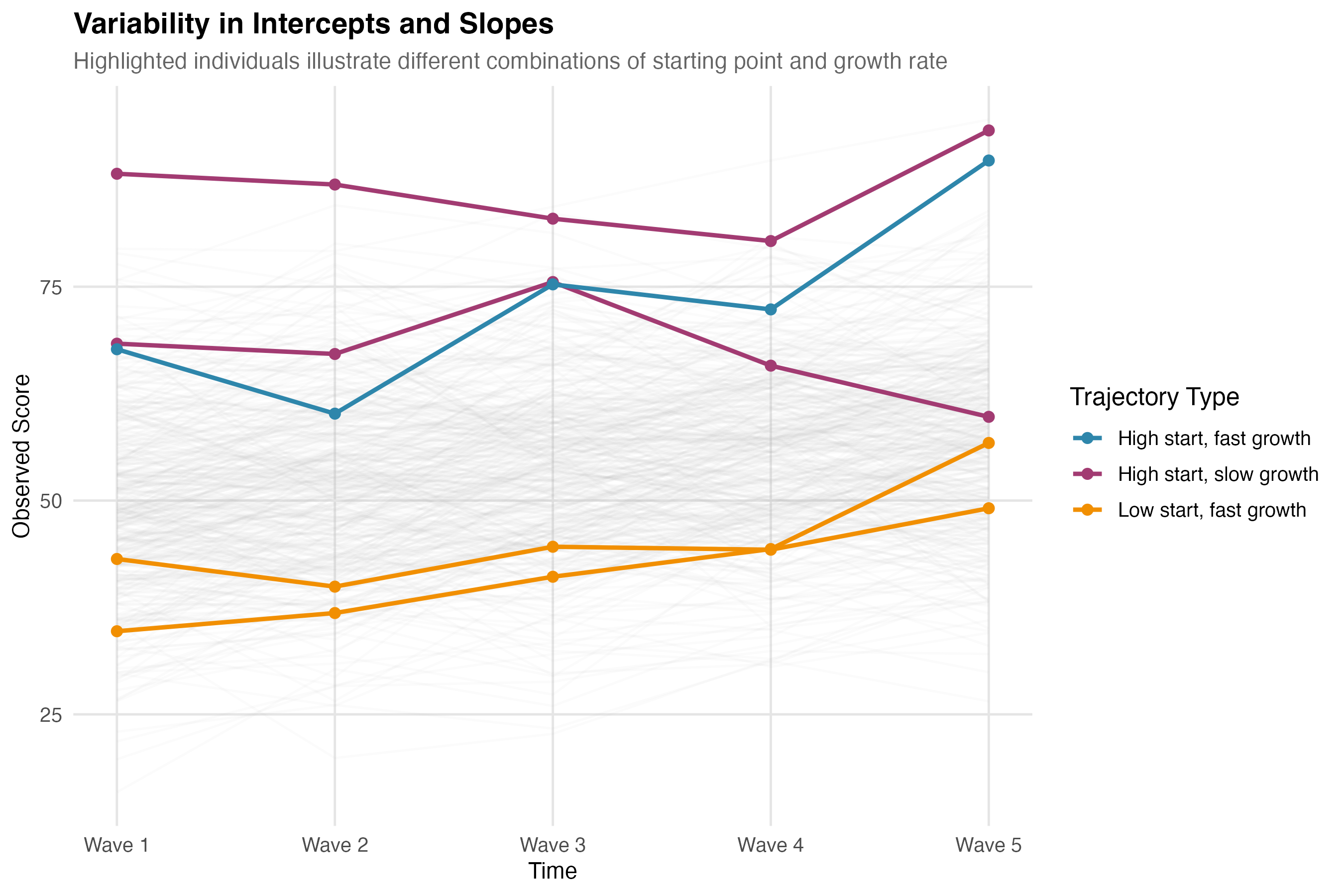
This figure illustrates three highlighted trajectories from different regions of the intercept-slope distribution:
| Trajectory | Intercept | Slope | Pattern |
|---|---|---|---|
| Blue | High | High | Started high, grew fast |
| Purple | High | Low | Started high, grew slowly |
| Orange | Low | High | Started low, grew fast |
The intercept-slope covariance determines how concentrated trajectories are in certain regions. A strong negative covariance would mean most people fall in the purple (high-low) and orange (low-high) patterns—high starters tend to grow slower, while low starters catch up.
Interactive Exploration
To build deeper intuition for how LGCM parameters affect trajectories, use the interactive explorer below. Adjust the sliders to see how changing the intercept mean, slope variance, and other parameters affects the spaghetti plot in real-time.
Practical Considerations
How Many Time Points?
LGCM requires at least 3 time points for linear growth, with 4+ preferred. With only two waves, simpler approaches (change scores, ANCOVA) work just as well. More waves provide better power to detect individual differences in growth and to test whether linear trajectories actually fit.
With 3 waves, linear growth is identified but overall model fit is weakly testable. With 4 waves, you can begin to test linear vs. alternative forms (note: a quadratic model can be just-identified under common constraints).
Missing Data
Real longitudinal data almost always have missing observations. LGCM handles this gracefully through Full Information Maximum Likelihood (FIML), which uses all available data without listwise deletion.
The key assumption is Missing At Random (MAR): missingness can depend on observed variables, but not on the missing values themselves. If participants drop out because their unobserved scores are extreme (Missing Not At Random), estimates may be biased. Understanding this distinction helps you evaluate whether your missing data pattern is problematic.
FIML assumes MAR and correct model specification. Include auxiliary variables related to missingness (and the outcome) to bolster MAR plausibility and reduce bias.
Time Coding
Slope factor loadings define how time enters the model. This determines:
- What the intercept represents
- How to interpret the slope
- Whether unequal spacing is handled correctly
Standard Coding (0, 1, 2, 3, 4)
| Wave | Loading | Meaning |
|---|---|---|
| 1 | 0 | Intercept = expected score here |
| 2 | 1 | 1 unit of time elapsed |
| 3 | 2 | 2 units elapsed |
| 4 | 3 | 3 units elapsed |
| 5 | 4 | 4 units elapsed |
With this coding:
- Intercept = expected score at Time 0 (Wave 1)
- Slope = expected change per 1-unit increase in time
Centering at Different Time Points
Shift the zero point to change what the intercept represents:
| Centering | Loadings | Intercept Meaning |
|---|---|---|
| Wave 1 (standard) | 0, 1, 2, 3, 4 | Expected score at Wave 1 |
| Midpoint (Wave 3) | -2, -1, 0, 1, 2 | Expected score at Wave 3 |
| Final (Wave 5) | -4, -3, -2, -1, 0 | Expected score at Wave 5 |

How time coding determines the intercept's location. All three panels show the same trajectory, but the intercept (marked "I") refers to different time points depending on where you place the zero in your slope loadings. The slope (rate of change) remains identical across all three.
Three panels showing the same linear trajectory with different intercept locations. Left (Wave 1 centering): Loadings 0,1,2,3,4 — intercept marked at Wave 1. Center (Midpoint centering): Loadings -2,-1,0,1,2 — intercept marked at Wave 3. Right (Final wave centering): Loadings -4,-3,-2,-1,0 — intercept marked at Wave 5. The slope (line angle) is identical in all three; only the intercept reference point changes.
Across different centerings, the meaning of the slope does not change; only the intercept's meaning shifts to the chosen time origin.
When does centering matter? When you add predictors. If you ask "Does baseline depression predict growth?", the intercept-predictor relationship depends on where you defined the intercept.
Non-Equidistant Time Points
If waves aren't equally spaced, use actual time values:
| Assessment | Time | Loading |
|---|---|---|
| Baseline | Month 0 | 0 |
| Follow-up 1 | Month 3 | 3 |
| Follow-up 2 | Month 6 | 6 |
| Follow-up 3 | Month 12 | 12 |
| Follow-up 4 | Month 24 | 24 |
Now slope = change per month. Rescale for interpretability if needed (e.g., divide by 12 for slope = change per year).
Rescaling the time metric also rescales the slope mean and variance (e.g., per-month → per-year), which can improve interpretability and numerical stability.
Common Pitfalls
| Pitfall | Mistake | Fix |
|---|---|---|
| Ignoring slope variance | "Everyone improved" (mean slope = 2) | If slope SD = 2, ~16% have slopes ≤ 0. Always report variance alongside the mean |
| Misreading I-S correlation | Negative correlation = high starters declined | Negative correlation = high starters grew slower. Combine with slope mean for direction |
| Confusing means with individuals | "The model shows steady improvement" | The mean summarizes the group; individual trajectories can differ wildly. Plot spaghetti plots |
| Equating good fit with truth | RMSEA < .06 proves the model is correct | Good fit = plausible, not true. Always compare alternatives (quadratic, piecewise) |
| Misinterpreting recentered intercepts | Recentered at midpoint but interpreted as "baseline" | The intercept refers to wherever time = 0 in your coding. Match interpretation to coding |
| Ignoring residual autocorrelation | Assumed residuals are independent without checking | Poor fit (or large modification indices) may indicate carryover effects. Consider autoregressive structures |
| Overfitting with too few waves | Quadratic model with 4 waves (0 df) | Just-identified models fit perfectly by construction. Ensure positive degrees of freedom |
| Ignoring missing data mechanism | Used FIML and assumed everything is fine | FIML assumes MAR. If dropout depends on unobserved values (MNAR), estimates may be biased. Include auxiliary variables |
| Over-interpreting non-significant variance | Slope variance p = .08, so "no differences" | You may be underpowered. Report the estimate and CI, not just the p-value |
| Forgetting to look at the data | Jumped straight to modeling | You might miss outliers, nonlinearity, or subgroups. Always plot spaghetti plots first |
Summary
You now have the conceptual foundation for understanding LGCM:
- Two latent factors—intercept and slope—capture each person's starting level and rate of change
- Factor variances quantify individual differences; the covariance reveals whether high starters grow faster or slower
- Time coding determines what the intercept means and must match your study design
- LGCM produces testable fit, allowing you to evaluate whether linear growth actually describes your data
This is enough to understand what an LGCM does and why. To actually fit one, continue to the worked example.
This hub focuses on linear LGCM for continuous outcomes. Not covered (yet): generalized growth for counts/binary, mixture/latent class growth, piecewise/latent-basis models, and measurement invariance testing when outcomes are latent factors measured by multiple items. See the tutorial links for code and estimation details.
Next Steps
Walkthrough: Worked Example → Step-by-step R code to simulate data, fit models, and interpret results.